1. Python and Pandas

1.1. Overview

This chapter provides an introduction to data science and the Python programming language. The goal here is to get your hands dirty right from the start! We will walk through an entire data analysis, and along the way introduce different types of data analysis question, some fundamental programming concepts in Python, and the basics of loading, cleaning, and visualizing data. In the following chapters, we will dig into each of these steps in much more detail; but for now, let’s jump in to see how much we can do with data science!

1.2. Chapter learning objectives

By the end of the chapter, readers will be able to do the following:

• Identify the different types of data analysis question and categorize a question into the correct type.

• Load the pandas package into Python.

• Read tabular data with read_csv.

• Create new variables and objects in Python using the assignment symbol.

• Create and organize subsets of tabular data using [], loc[], sort_values, and head.

• Add and modify columns in tabular data using column assignment.

• Chain multiple operations in sequence.

• Visualize data with an altair bar plot.

• Use help() and ? to access help and documentation tools in Python.

1.3. Canadian languages data set

In this chapter, we will walk through a full analysis of a data set relating to languages spoken at home by Canadian residents (Fig. 1.1). Many Indigenous peoples exist in Canada with their own cultures and languages; these languages are often unique to Canada and not spoken anywhere else in the world [Statistics Canada, 2018]. Sadly, colonization has led to the loss of many of these languages. For instance, generations of children were not allowed to speak their mother tongue (the first language an individual learns in childhood) in Canadian residential schools. Colonizers also renamed places they had “discovered” [Wilson, 2018]. Acts such as these have significantly harmed the continuity of Indigenous languages in Canada, and some languages are considered “endangered” as few people report speaking them. To learn more, please see Canadian Geographic’s article, “Mapping Indigenous Languages in Canada” [Walker, 2017], They Came for the Children: Canada, Aboriginal peoples, and Residential Schools [Truth and Reconciliation Commission of Canada, 2012] and the Truth and Reconciliation Commission of Canada’s Calls to Action [Truth and Reconciliation Commission of Canada, 2015].

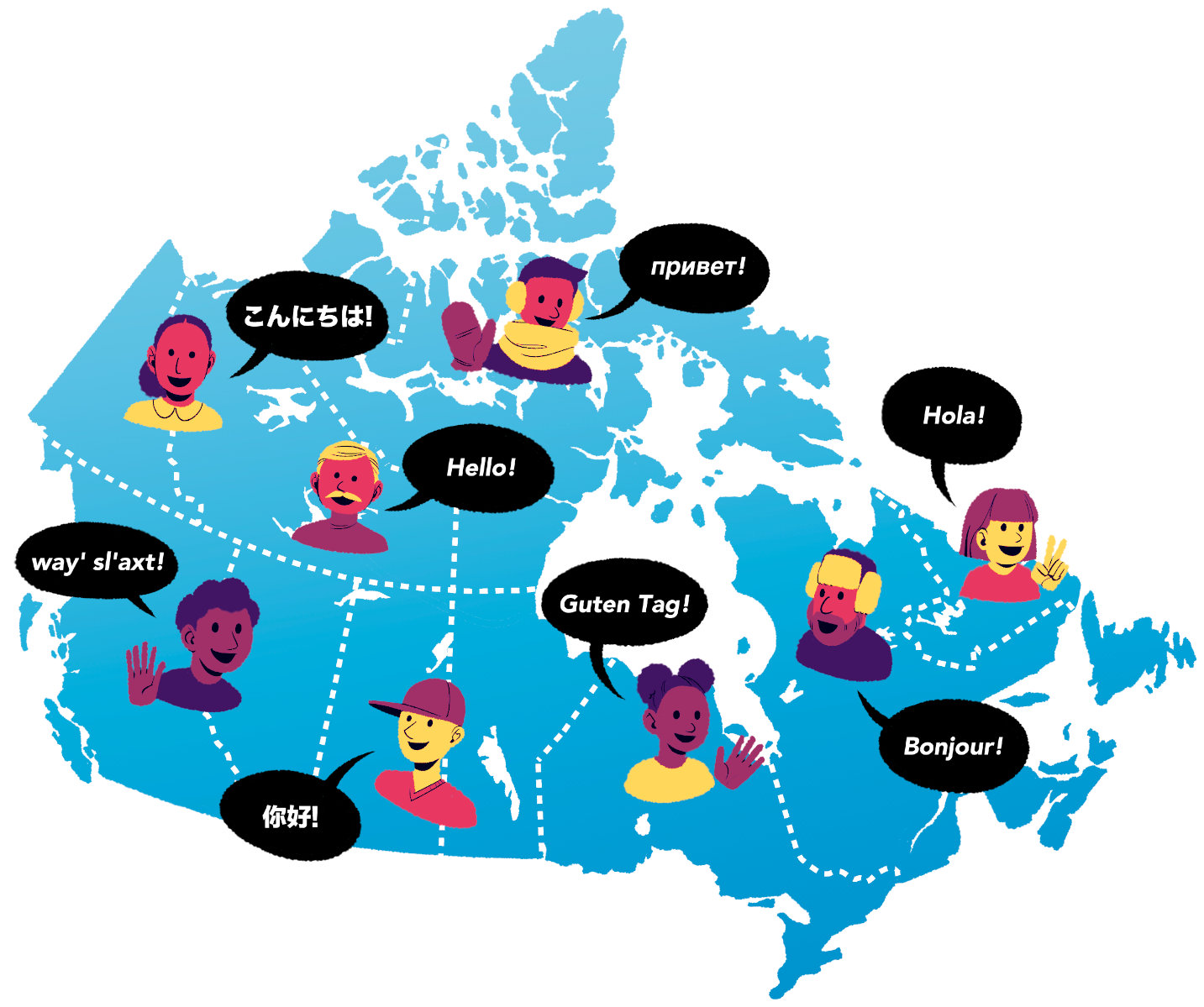
Fig. 1.1 Map of Canada

The data set we will study in this chapter is taken from the canlang R data package [Timbers, 2020], which has population language data collected during the 2016 Canadian census [Statistics Canada, 2016]. In this data, there are 214 languages recorded, each having six different properties:

1. category: Higher-level language category, describing whether the language is an Official Canadian language, an Aboriginal (i.e., Indigenous) language, or a Non-Official and Non-Aboriginal language.

2. language: The name of the language.

3. mother_tongue: Number of Canadian residents who reported the language as their mother tongue. Mother tongue is generally defined as the language someone was exposed to since birth.

4. most_at_home: Number of Canadian residents who reported the language as being spoken most often at home.

5. most_at_work: Number of Canadian residents who reported the language as being used most often at work.

6. lang_known: Number of Canadian residents who reported knowledge of the language.

According to the census, more than 60 Aboriginal languages were reported as being spoken in Canada. Suppose we want to know which are the most common; then we might ask the following question, which we wish to answer using our data:

Which ten Aboriginal languages were most often reported in 2016 as mother tongues in Canada, and how many people speak each of them?

Note

Data science cannot be done without a deep understanding of the data and problem domain. In this book, we have simplified the data sets used in our examples to concentrate on methods and fundamental concepts. But in real life, you cannot and should not do data science without a domain expert. Alternatively, it is common to practice data science in your own domain of expertise! Remember that when you work with data, it is essential to think about how the data were collected, which affects the conclusions you can draw. If your data are biased, then your results will be biased!

1.4. Asking a question

Every good data analysis begins with a question—like the above—that you aim to answer using data. As it turns out, there are actually a number of different types of question regarding data: descriptive, exploratory, predictive, inferential, causal, and mechanistic, all of which are defined in Table 1.1. [Leek and Peng, 2015, Peng and Matsui, 2015] Carefully formulating a question as early as possible in your analysis—and correctly identifying which type of question it is—will guide your overall approach to the analysis as well as the selection of appropriate tools.

Table 1.1 Types of data analysis question.

Question type	Description	Example
Descriptive	A question that asks about summarized characteristics of a data set without interpretation (i.e., report a fact).	How many people live in each province and territory in Canada?
Exploratory	A question that asks if there are patterns, trends, or relationships within a single data set. Often used to propose hypotheses for future study.	Does political party voting change with indicators of wealth in a set of data collected on 2,000 people living in Canada?
Predictive	A question that asks about predicting measurements or labels for individuals (people or things). The focus is on what things predict some outcome, but not what causes the outcome.	What political party will someone vote for in the next Canadian election?
Inferential	A question that looks for patterns, trends, or relationships in a single data set and also asks for quantification of how applicable these findings are to the wider population.	Does political party voting change with indicators of wealth for all people living in Canada?
Causal	A question that asks about whether changing one factor will lead to a change in another factor, on average, in the wider population.	Does wealth lead to voting for a certain political party in Canadian elections?
Mechanistic	A question that asks about the underlying mechanism of the observed patterns, trends, or relationships (i.e., how does it happen?)	How does wealth lead to voting for a certain political party in Canadian elections?

In this book, you will learn techniques to answer the first four types of question: descriptive, exploratory, predictive, and inferential; causal and mechanistic questions are beyond the scope of this book. In particular, you will learn how to apply the following analysis tools:

1. Summarization: computing and reporting aggregated values pertaining to a data set. Summarization is most often used to answer descriptive questions, and can occasionally help with answering exploratory questions. For example, you might use summarization to answer the following question: What is the average race time for runners in this data set? Tools for summarization are covered in detail in Chapters 2 and 3, but appear regularly throughout the text.

2. Visualization: plotting data graphically. Visualization is typically used to answer descriptive and exploratory questions, but plays a critical supporting role in answering all of the types of question in Table 1.1. For example, you might use visualization to answer the following question: Is there any relationship between race time and age for runners in this data set? This is covered in detail in Chapter 4, but again appears regularly throughout the book.

3. Classification: predicting a class or category for a new observation. Classification is used to answer predictive questions. For example, you might use classification to answer the following question: Given measurements of a tumor’s average cell area and perimeter, is the tumor benign or malignant? Classification is covered in Chapters 5 and 6.

4. Regression: predicting a quantitative value for a new observation. Regression is also used to answer predictive questions. For example, you might use regression to answer the following question: What will be the race time for a 20-year-old runner who weighs 50kg? Regression is covered in Chapters 7 and 8.

5. Clustering: finding previously unknown/unlabeled subgroups in a data set. Clustering is often used to answer exploratory questions. For example, you might use clustering to answer the following question: What products are commonly bought together on Amazon? Clustering is covered in Chapter 9.

6. Estimation: taking measurements for a small number of items from a large group and making a good guess for the average or proportion for the large group. Estimation is used to answer inferential questions. For example, you might use estimation to answer the following question: Given a survey of cellphone ownership of 100 Canadians, what proportion of the entire Canadian population own Android phones? Estimation is covered in Chapter 10.

Referring to Table 1.1, our question about Aboriginal languages is an example of a descriptive question: we are summarizing the characteristics of a data set without further interpretation. And referring to the list above, it looks like we should use visualization and perhaps some summarization to answer the question. So in the remainder of this chapter, we will work towards making a visualization that shows us the ten most common Aboriginal languages in Canada and their associated counts, according to the 2016 census.

1.5. Loading a tabular data set

A data set is, at its core essence, a structured collection of numbers and characters. Aside from that, there are really no strict rules; data sets can come in many different forms! Perhaps the most common form of data set that you will find in the wild, however, is tabular data. Think spreadsheets in Microsoft Excel: tabular data are rectangular-shaped and spreadsheet-like, as shown in Fig. 1.2. In this book, we will focus primarily on tabular data.

Since we are using Python for data analysis in this book, the first step for us is to load the data into Python. When we load tabular data into Python, it is represented as a data frame object. Fig. 1.2 shows that a Python data frame is very similar to a spreadsheet. We refer to the rows as observations; these are the individual objects for which we collect data. In Fig. 1.2, the observations are languages. We refer to the columns as variables; these are the characteristics of each observation. In Fig. 1.2, the variables are the the language’s category, its name, the number of mother tongue speakers, etc.

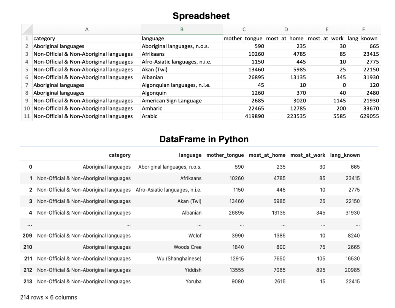
Fig. 1.2 A spreadsheet versus a data frame in Python

The first kind of data file that we will learn how to load into Python as a data frame is the comma-separated values format (.csv for short). These files have names ending in .csv, and can be opened and saved using common spreadsheet programs like Microsoft Excel and Google Sheets. For example, the .csv file named can_lang.csv is included with the code for this book. If we were to open this data in a plain text editor (a program like Notepad that just shows text with no formatting), we would see each row on its own line, and each entry in the table separated by a comma:

category,language,mother_tongue,most_at_home,most_at_work,lang_known
Aboriginal languages,"Aboriginal languages, n.o.s.",590,235,30,665
Non-Official & Non-Aboriginal languages,Afrikaans,10260,4785,85,23415
Non-Official & Non-Aboriginal languages,"Afro-Asiatic languages, n.i.e.",1150,44
Non-Official & Non-Aboriginal languages,Akan (Twi),13460,5985,25,22150
Non-Official & Non-Aboriginal languages,Albanian,26895,13135,345,31930
Aboriginal languages,"Algonquian languages, n.i.e.",45,10,0,120
Aboriginal languages,Algonquin,1260,370,40,2480
Non-Official & Non-Aboriginal languages,American Sign Language,2685,3020,1145,21
Non-Official & Non-Aboriginal languages,Amharic,22465,12785,200,33670

To load this data into Python so that we can do things with it (e.g., perform analyses or create data visualizations), we will need to use a function. A function is a special word in Python that takes instructions (we call these arguments) and does something. The function we will use to load a .csv file into Python is called read_csv. In its most basic use-case, read_csv expects that the data file:

• has column names (or headers),

• uses a comma (,) to separate the columns, and

• does not have row names.

Below you’ll see the code used to load the data into Python using the read_csv function. Note that the read_csv function is not included in the base installation of Python, meaning that it is not one of the primary functions ready to use when you install Python. Therefore, you need to load it from somewhere else before you can use it. The place from which we will load it is called a Python package. A Python package is a collection of functions that can be used in addition to the built-in Python package functions once loaded. The read_csv function, in particular, can be made accessible by loading the pandas Python package [The Pandas Development Team, 2020, Wes McKinney, 2010] using the import command. The pandas package contains many functions that we will use throughout this book to load, clean, wrangle, and visualize data.

import pandas as pd

This command has two parts. The first is import pandas, which loads the pandas package. The second is as pd, which give the pandas package the much shorter alias (another name) pd. We can now use the read_csv function by writing pd.read_csv, i.e., the package name, then a dot, then the function name. You can see why we gave pandas a shorter alias; if we had to type pandas. before every function we wanted to use, our code would become much longer and harder to read!

Now that the pandas package is loaded, we can use the read_csv function by passing it a single argument: the name of the file, "can_lang.csv". We have to put quotes around file names and other letters and words that we use in our code to distinguish it from the special words (like functions!) that make up the Python programming language. The file’s name is the only argument we need to provide because our file satisfies everything else that the read_csv function expects in the default use-case. Fig. 1.3 describes how we use the read_csv to read data into Python.

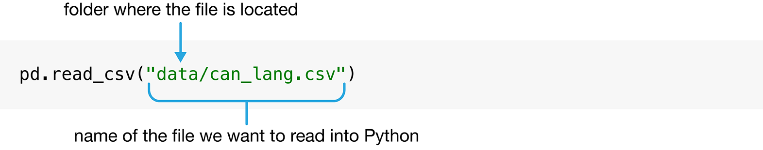
Fig. 1.3 Syntax for the read_csv function

pd.read_csv("data/can_lang.csv")

	category	language	mother_tongue	most_at_home	most_at_work	lang_known
0	Aboriginal languages	Aboriginal languages, n.o.s.	590	235	30	665
1	Non-Official & Non-Aboriginal languages	Afrikaans	10260	4785	85	23415
2	Non-Official & Non-Aboriginal languages	Afro-Asiatic languages, n.i.e.	1150	445	10	2775
3	Non-Official & Non-Aboriginal languages	Akan (Twi)	13460	5985	25	22150
4	Non-Official & Non-Aboriginal languages	Albanian	26895	13135	345	31930
...	...	...	...	...	...	...
209	Non-Official & Non-Aboriginal languages	Wolof	3990	1385	10	8240
210	Aboriginal languages	Woods Cree	1840	800	75	2665
211	Non-Official & Non-Aboriginal languages	Wu (Shanghainese)	12915	7650	105	16530
212	Non-Official & Non-Aboriginal languages	Yiddish	13555	7085	895	20985
213	Non-Official & Non-Aboriginal languages	Yoruba	9080	2615	15	22415

214 rows × 6 columns

1.6. Naming things in Python

When we loaded the 2016 Canadian census language data using read_csv, we did not give this data frame a name. Therefore the data was just printed on the screen, and we cannot do anything else with it. That isn’t very useful. What would be more useful would be to give a name to the data frame that read_csv outputs, so that we can refer to it later for analysis and visualization.

The way to assign a name to a value in Python is via the assignment symbol =. On the left side of the assignment symbol you put the name that you want to use, and on the right side of the assignment symbol you put the value that you want the name to refer to. Names can be used to refer to almost anything in Python, such as numbers, words (also known as strings of characters), and data frames! Below, we set my_number to 3 (the result of 1+2) and we set name to the string "Alice".

my_number = 1 + 2
name = "Alice"

Note that when we name something in Python using the assignment symbol, =, we do not need to surround the name we are creating with quotes. This is because we are formally telling Python that this special word denotes the value of whatever is on the right-hand side. Only characters and words that act as values on the right-hand side of the assignment symbol—e.g., the file name "data/can_lang.csv" that we specified before, or "Alice" above—need to be surrounded by quotes.

After making the assignment, we can use the special name words we have created in place of their values. For example, if we want to do something with the value 3 later on, we can just use my_number instead. Let’s try adding 2 to my_number; you will see that Python just interprets this as adding 2 and 3:

my_number + 2

5

Object names can consist of letters, numbers, and underscores (_). Other symbols won’t work since they have their own meanings in Python. For example, - is the subtraction symbol; if we try to assign a name with the - symbol, Python will complain and we will get an error!

my-number = 1

SyntaxError: cannot assign to expression here. Maybe you meant '==' instead of '='?

There are certain conventions for naming objects in Python. When naming an object we suggest using only lowercase letters, numbers and underscores _ to separate the words in a name. Python is case sensitive, which means that Letter and letter would be two different objects in Python. You should also try to give your objects meaningful names. For instance, you can name a data frame x. However, using more meaningful terms, such as language_data, will help you remember what each name in your code represents. We recommend following the PEP 8 naming conventions outlined in the PEP 8 [Guido van Rossum, 2001]. Let’s now use the assignment symbol to give the name can_lang to the 2016 Canadian census language data frame that we get from read_csv.

can_lang = pd.read_csv("data/can_lang.csv")

Wait a minute, nothing happened this time! Where’s our data? Actually, something did happen: the data was loaded in and now has the name can_lang associated with it. And we can use that name to access the data frame and do things with it. For example, we can type the name of the data frame to print both the first few rows and the last few rows. The three dots (...) indicate that there are additional rows that are not printed. You will also see that the number of observations (i.e., rows) and variables (i.e., columns) are printed just underneath the data frame (214 rows and 6 columns in this case). Printing a few rows from data frame like this is a handy way to get a quick sense for what is contained in it.

can_lang

	category	language	mother_tongue	most_at_home	most_at_work	lang_known
0	Aboriginal languages	Aboriginal languages, n.o.s.	590	235	30	665
1	Non-Official & Non-Aboriginal languages	Afrikaans	10260	4785	85	23415
2	Non-Official & Non-Aboriginal languages	Afro-Asiatic languages, n.i.e.	1150	445	10	2775
3	Non-Official & Non-Aboriginal languages	Akan (Twi)	13460	5985	25	22150
4	Non-Official & Non-Aboriginal languages	Albanian	26895	13135	345	31930
...	...	...	...	...	...	...
209	Non-Official & Non-Aboriginal languages	Wolof	3990	1385	10	8240
210	Aboriginal languages	Woods Cree	1840	800	75	2665
211	Non-Official & Non-Aboriginal languages	Wu (Shanghainese)	12915	7650	105	16530
212	Non-Official & Non-Aboriginal languages	Yiddish	13555	7085	895	20985
213	Non-Official & Non-Aboriginal languages	Yoruba	9080	2615	15	22415

214 rows × 6 columns

1.7. Creating subsets of data frames with [] & loc[]

Now that we’ve loaded our data into Python, we can start wrangling the data to find the ten Aboriginal languages that were most often reported in 2016 as mother tongues in Canada. In particular, we want to construct a table with the ten Aboriginal languages that have the largest counts in the mother_tongue column. The first step is to extract from our can_lang data only those rows that correspond to Aboriginal languages, and then the second step is to keep only the language and mother_tongue columns. The [] and loc[] operations on the pandas data frame will help us here. The [] allows you to obtain a subset of (i.e., filter) the rows of a data frame, or to obtain a subset of (i.e., select) the columns of a data frame. The loc[] operation allows you to both filter rows and select columns at the same time. We will first investigate filtering rows and selecting columns with the [] operation, and then use loc[] to do both in our analysis of the Aboriginal languages data.

Note

The [] and loc[] operations, and related operations, in pandas are much more powerful than we describe in this chapter. You will learn more sophisticated ways to index data frames later on in Chapter 3.

1.7.1. Using [] to filter rows

Looking at the can_lang data above, we see the column category contains different high-level categories of languages, which include “Aboriginal languages”, “Non-Official & Non-Aboriginal languages” and “Official languages”. To answer our question we want to filter our data set so we restrict our attention to only those languages in the “Aboriginal languages” category.

We can use the [] operation to obtain the subset of rows with desired values from a data frame. Fig. 1.4 shows the syntax we need to use to filter rows with the [] operation. First, we type the name of the data frame—here, can_lang—followed by square brackets. Inside the square brackets, we write a logical statement to use when filtering the rows. A logical statement evaluates to either True or False for each row in the data frame; the [] operation keeps only those rows for which the logical statement evaluates to True. For example, in our analysis, we are interested in keeping only languages in the "Aboriginal languages" higher-level category. We can use the equivalency operator == to compare the values of the category column—denoted by can_lang["category"]—with the value "Aboriginal languages". You will learn about many other kinds of logical statement in Chapter 3. Similar to when we loaded the data file and put quotes around the file name, here we need to put quotes around both "Aboriginal languages" and "category". Using quotes tells Python that this is a string value (e.g., a column name, or word data) and not one of the special words that make up the Python programming language, or one of the names we have given to objects in the code we have already written.

Note

In Python, single quotes (') and double quotes (") are generally treated the same. So we could have written 'Aboriginal languages' instead of "Aboriginal languages" above, or 'category' instead of "category". Try both out for yourself!

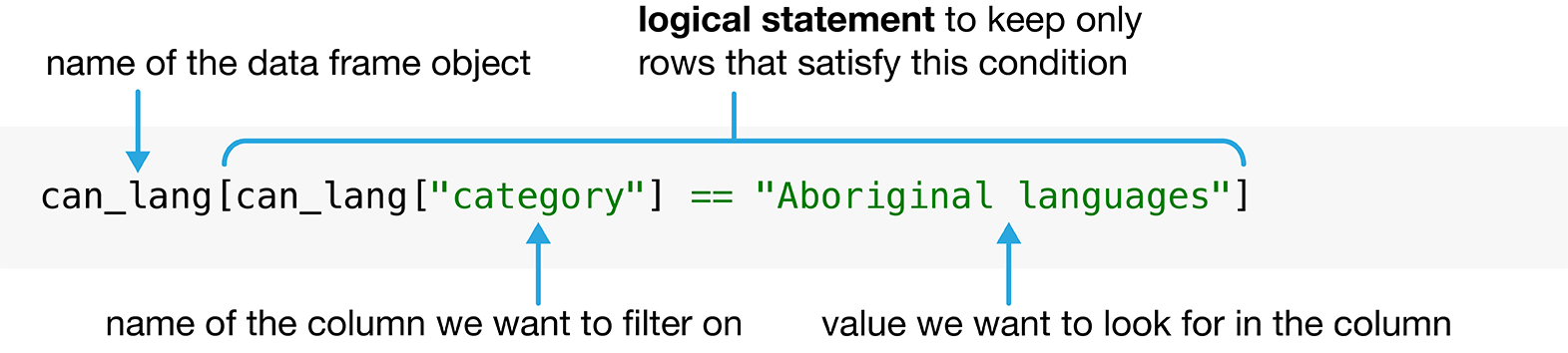
Fig. 1.4 Syntax for using the [] operation to filter rows.

This operation returns a data frame that has all the columns of the input data frame, but only those rows corresponding to Aboriginal languages that we asked for in the logical statement.

can_lang[can_lang["category"] == "Aboriginal languages"]

	category	language	mother_tongue	most_at_home	most_at_work	lang_known
0	Aboriginal languages	Aboriginal languages, n.o.s.	590	235	30	665
5	Aboriginal languages	Algonquian languages, n.i.e.	45	10	0	120
6	Aboriginal languages	Algonquin	1260	370	40	2480
12	Aboriginal languages	Athabaskan languages, n.i.e.	50	10	0	85
13	Aboriginal languages	Atikamekw	6150	5465	1100	6645
...	...	...	...	...	...	...
191	Aboriginal languages	Thompson (Ntlakapamux)	335	20	0	450
195	Aboriginal languages	Tlingit	95	0	10	260
196	Aboriginal languages	Tsimshian	200	30	10	410
206	Aboriginal languages	Wakashan languages, n.i.e.	10	0	0	25
210	Aboriginal languages	Woods Cree	1840	800	75	2665

67 rows × 6 columns

1.7.2. Using [] to select columns

We can also use the [] operation to select columns from a data frame. Fig. 1.5 displays the syntax needed to select columns. We again first type the name of the data frame—here, can_lang—followed by square brackets. Inside the square brackets, we provide a list of column names. In Python, we denote a list using square brackets, where each item is separated by a comma (,). So if we are interested in selecting only the language and mother_tongue columns from our original can_lang data frame, we put the list ["language", "mother_tongue"] containing those two column names inside the square brackets of the [] operation.

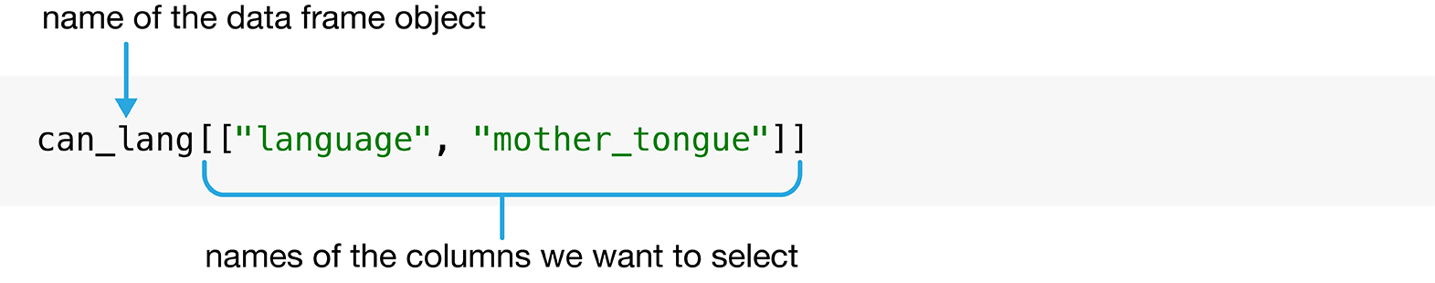
Fig. 1.5 Syntax for using the [] operation to select columns.

This operation returns a data frame that has all the rows of the input data frame, but only those columns that we named in the selection list.

can_lang[["language", "mother_tongue"]]

	language	mother_tongue
0	Aboriginal languages, n.o.s.	590
1	Afrikaans	10260
2	Afro-Asiatic languages, n.i.e.	1150
3	Akan (Twi)	13460
4	Albanian	26895
...	...	...
209	Wolof	3990
210	Woods Cree	1840
211	Wu (Shanghainese)	12915
212	Yiddish	13555
213	Yoruba	9080

214 rows × 2 columns

1.7.3. Using loc[] to filter rows and select columns

The [] operation is only used when you want to filter rows or select columns; it cannot be used to do both operations at the same time. But in order to answer our original data analysis question in this chapter, we need to both filter the rows for Aboriginal languages, and select the language and mother_tongue columns. Fortunately, pandas provides the loc[] operation, which lets us do just that. The syntax is very similar to the [] operation we have already covered: we will essentially combine both our row filtering and column selection steps from before. In particular, we first write the name of the data frame—can_lang again—then follow that with the .loc[] operation. Inside the square brackets, we write our row filtering logical statement, then a comma, then our list of columns to select.

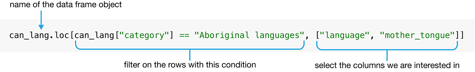
Fig. 1.6 Syntax for using the loc[] operation to filter rows and select columns.

aboriginal_lang = can_lang.loc[can_lang["category"] == "Aboriginal languages", ["language", "mother_tongue"]]

There is one very important thing to notice in this code example. The first is that we used the loc[] operation on the can_lang data frame by writing can_lang.loc[]—first the data frame name, then a dot, then loc[]. There’s that dot again! If you recall, earlier in this chapter we used the read_csv function from pandas (aliased as pd), and wrote pd.read_csv. The dot means that the thing on the left (pd, i.e., the pandas package) provides the thing on the right (the read_csv function). In the case of can_lang.loc[], the thing on the left (the can_lang data frame) provides the thing on the right (the loc[] operation). In Python, both packages (like pandas) and objects (like our can_lang data frame) can provide functions and other objects that we access using the dot syntax.

Note

A note on terminology: when an object obj provides a function f with the dot syntax (as in obj.f()), sometimes we call that function f a method of obj or an operation on obj. Similarly, when an object obj provides another object x with the dot syntax (as in obj.x), sometimes we call the object x an attribute of obj. We will use all of these terms throughout the book, as you will see them used commonly in the community. And just because we programmers like to be confusing for no apparent reason: we don’t use the “method”, “operation”, or “attribute” terminology when referring to functions and objects from packages, like pandas. So for example, pd.read_csv would typically just be referred to as a function, but not as a method or operation, even though it uses the dot syntax.

At this point, if we have done everything correctly, aboriginal_lang should be a data frame containing only rows where the category is "Aboriginal languages", and containing only the language and mother_tongue columns. Any time you take a step in a data analysis, it’s good practice to check the output by printing the result.

aboriginal_lang

	language	mother_tongue
0	Aboriginal languages, n.o.s.	590
5	Algonquian languages, n.i.e.	45
6	Algonquin	1260
12	Athabaskan languages, n.i.e.	50
13	Atikamekw	6150
...	...	...
191	Thompson (Ntlakapamux)	335
195	Tlingit	95
196	Tsimshian	200
206	Wakashan languages, n.i.e.	10
210	Woods Cree	1840

67 rows × 2 columns

We can see the original can_lang data set contained 214 rows with multiple kinds of category. The data frame aboriginal_lang contains only 67 rows, and looks like it only contains Aboriginal languages. So it looks like the loc[] operation gave us the result we wanted!

1.8. Using sort_values and head to select rows by ordered values

We have used the [] and loc[] operations on a data frame to obtain a table with only the Aboriginal languages in the data set and their associated counts. However, we want to know the ten languages that are spoken most often. As a next step, we will order the mother_tongue column from largest to smallest value and then extract only the top ten rows. This is where the sort_values and head functions come to the rescue!

The sort_values function allows us to order the rows of a data frame by the values of a particular column. We need to specify the column name by which we want to sort the data frame by passing it to the argument by. Since we want to choose the ten Aboriginal languages most often reported as a mother tongue language, we will use the sort_values function to order the rows in our selected_lang data frame by the mother_tongue column. We want to arrange the rows in descending order (from largest to smallest), so we specify the argument ascending as False.

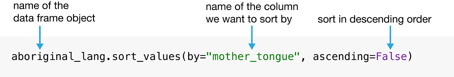
Fig. 1.7 Syntax for using sort_values to arrange rows in decending order.

arranged_lang = aboriginal_lang.sort_values(by="mother_tongue", ascending=False)
arranged_lang

	language	mother_tongue
40	Cree, n.o.s.	64050
89	Inuktitut	35210
138	Ojibway	17885
137	Oji-Cree	12855
48	Dene	10700
...	...	...
5	Algonquian languages, n.i.e.	45
32	Cayuga	45
179	Squamish	40
90	Iroquoian languages, n.i.e.	35
206	Wakashan languages, n.i.e.	10

67 rows × 2 columns

Next, we will obtain the ten most common Aboriginal languages by selecting only the first ten rows of the arranged_lang data frame. We do this using the head function, and specifying the argument 10.

ten_lang = arranged_lang.head(10)
ten_lang

	language	mother_tongue
40	Cree, n.o.s.	64050
89	Inuktitut	35210
138	Ojibway	17885
137	Oji-Cree	12855
48	Dene	10700
125	Montagnais (Innu)	10235
119	Mi'kmaq	6690
13	Atikamekw	6150
149	Plains Cree	3065
180	Stoney	3025

1.9. Adding and modifying columns

Recall that our data analysis question referred to the count of Canadians that speak each of the top ten most commonly reported Aboriginal languages as their mother tongue, and the ten_lang data frame indeed contains those counts… But perhaps, seeing these numbers, we became curious about the percentage of the population of Canada associated with each count. It is common to come up with new data analysis questions in the process of answering a first one—so fear not and explore! To answer this small question along the way, we need to divide each count in the mother_tongue column by the total Canadian population according to the 2016 census—i.e., 35,151,728—and multiply it by 100. We can perform this computation using the code 100 * ten_lang["mother_tongue"] / canadian_population. Then to store the result in a new column (or overwrite an existing column), we specify the name of the new column to create (or old column to modify), then the assignment symbol =, and then the computation to store in that column. In this case, we will opt to create a new column called mother_tongue_percent.

Note

You will see below that we write the Canadian population in Python as 35_151_728. The underscores (_) are just there for readability, and do not affect how Python interprets the number. In other words, 35151728 and 35_151_728 are treated identically in Python, although the latter is much clearer!

canadian_population = 35_151_728
ten_lang["mother_tongue_percent"] = 100 * ten_lang["mother_tongue"] / canadian_population
ten_lang

	language	mother_tongue	mother_tongue_percent
40	Cree, n.o.s.	64050	0.182210
89	Inuktitut	35210	0.100166
138	Ojibway	17885	0.050879
137	Oji-Cree	12855	0.036570
48	Dene	10700	0.030439
125	Montagnais (Innu)	10235	0.029117
119	Mi'kmaq	6690	0.019032
13	Atikamekw	6150	0.017496
149	Plains Cree	3065	0.008719
180	Stoney	3025	0.008606

The ten_lang_percent data frame shows that the ten Aboriginal languages in the ten_lang data frame were spoken as a mother tongue by between 0.008% and 0.18% of the Canadian population.

1.10. Combining steps with chaining and multiline expressions

It took us 3 steps to find the ten Aboriginal languages most often reported in 2016 as mother tongues in Canada. Starting from the can_lang data frame, we:

1. used loc to filter the rows so that only the Aboriginal languages category remained, and selected the language and mother_tongue columns,

2. used sort_values to sort the rows by mother_tongue in descending order, and

3. obtained only the top 10 values using head.

One way of performing these steps is to just write multiple lines of code, storing temporary, intermediate objects as you go.

aboriginal_lang = can_lang.loc[can_lang["category"] == "Aboriginal languages", ["language", "mother_tongue"]]
arranged_lang_sorted = aboriginal_lang.sort_values(by="mother_tongue", ascending=False)
ten_lang = arranged_lang_sorted.head(10)

You might find that code hard to read. You’re not wrong; it is! There are two main issues with readability here. First, each line of code is quite long. It is hard to keep track of what methods are being called, and what arguments were used. Second, each line introduces a new temporary object. In this case, both aboriginal_lang and arranged_lang_sorted are just temporary results on the way to producing the ten_lang data frame. This makes the code hard to read, as one has to trace where each temporary object goes, and hard to understand, since introducing many named objects also suggests that they are of some importance, when really they are just intermediates. The need to call multiple methods in a sequence to process a data frame is quite common, so this is an important issue to address!

To solve the first problem, we can actually split the long expressions above across multiple lines. Although in most cases, a single expression in Python must be contained in a single line of code, there are a small number of situations where lets us do this. Let’s rewrite this code in a more readable format using multiline expressions.

aboriginal_lang = can_lang.loc[
    can_lang["category"] == "Aboriginal languages",
    ["language", "mother_tongue"]
]
arranged_lang_sorted = aboriginal_lang.sort_values(
    by="mother_tongue",
    ascending=False
)
ten_lang = arranged_lang_sorted.head(10)

This code is the same as the code we showed earlier; you can see the same sequence of methods and arguments is used. But long expressions are split across multiple lines when they would otherwise get long and unwieldy, improving the readability of the code. How does Python know when to keep reading on the next line for a single expression? For the line starting with aboriginal_lang = ..., Python sees that the line ends with a left bracket symbol [, and knows that our expression cannot end until we close it with an appropriate corresponding right bracket symbol ]. We put the same two arguments as we did before, and then the corresponding right bracket appears after ["language", "mother_tongue"]). For the line starting with arranged_lang_sorted = ..., Python sees that the line ends with a left parenthesis symbol (, and knows the expression cannot end until we close it with the corresponding right parenthesis symbol ). Again we use the same two arguments as before, and then the corresponding right parenthesis appears right after ascending=False. In both cases, Python keeps reading the next line to figure out what the rest of the expression is. We could, of course, put all of the code on one line of code, but splitting it across multiple lines helps a lot with code readability.

We still have to handle the issue that each line of code—i.e., each step in the analysis—introduces a new temporary object. To address this issue, we can chain multiple operations together without assigning intermediate objects. The key idea of chaining is that the output of each step in the analysis is a data frame, which means that you can just directly keep calling methods that operate on the output of each step in a sequence! This simplifies the code and makes it easier to read. The code below demonstrates the use of both multiline expressions and chaining together. The code is now much cleaner, and the ten_lang data frame that we get is equivalent to the one from the messy code above!

# obtain the 10 most common Aboriginal languages
ten_lang = (
    can_lang.loc[
       can_lang["category"] == "Aboriginal languages",
       ["language", "mother_tongue"]
    ]
    .sort_values(by="mother_tongue", ascending=False)
    .head(10)
)
ten_lang

	language	mother_tongue
40	Cree, n.o.s.	64050
89	Inuktitut	35210
138	Ojibway	17885
137	Oji-Cree	12855
48	Dene	10700
125	Montagnais (Innu)	10235
119	Mi'kmaq	6690
13	Atikamekw	6150
149	Plains Cree	3065
180	Stoney	3025

Let’s parse this new block of code piece by piece. The code above starts with a left parenthesis, (, and so Python knows to keep reading to subsequent lines until it finds the corresponding right parenthesis symbol ). The loc method performs the filtering and selecting steps as before. The line after this starts with a period (.) that “chains” the output of the loc step with the next operation, sort_values. Since the output of loc is a data frame, we can use the sort_values method on it without first giving it a name! That is what the .sort_values does on the next line. Finally, we once again “chain” together the output of sort_values with head to ask for the 10 most common languages. Finally, the right parenthesis ) corresponding to the very first left parenthesis appears on the second last line, completing the multiline expression. Instead of creating intermediate objects, with chaining, we take the output of one operation and use that to perform the next operation. In doing so, we remove the need to create and store intermediates. This can help with readability by simplifying the code.

Now that we’ve shown you chaining as an alternative to storing temporary objects and composing code, does this mean you should never store temporary objects or compose code? Not necessarily! There are times when temporary objects are handy to keep around. For example, you might store a temporary object before feeding it into a plot function so you can iteratively change the plot without having to redo all of your data transformations. Chaining many functions can be overwhelming and difficult to debug; you may want to store a temporary object midway through to inspect your result before moving on with further steps.

1.11. Exploring data with visualizations

The ten_lang table answers our initial data analysis question. Are we done? Well, not quite; tables are almost never the best way to present the result of your analysis to your audience. Even the ten_lang table with only two columns presents some difficulty: for example, you have to scrutinize the table quite closely to get a sense for the relative numbers of speakers of each language. When you move on to more complicated analyses, this issue only gets worse. In contrast, a visualization would convey this information in a much more easily understood format. Visualizations are a great tool for summarizing information to help you effectively communicate with your audience, and creating effective data visualizations is an essential component of any data analysis. In this section we will develop a visualization of the ten Aboriginal languages that were most often reported in 2016 as mother tongues in Canada, as well as the number of people that speak each of them.

1.11.1. Using altair to create a bar plot

In our data set, we can see that language and mother_tongue are in separate columns (or variables). In addition, there is a single row (or observation) for each language. The data are, therefore, in what we call a tidy data format. Tidy data is a fundamental concept and will be a significant focus in the remainder of this book: many of the functions from pandas require tidy data, as does the altair package that we will use shortly for our visualization. We will formally introduce tidy data in Chapter 3.

We will make a bar plot to visualize our data. A bar plot is a chart where the lengths of the bars represent certain values, like counts or proportions. We will make a bar plot using the mother_tongue and language columns from our ten_lang data frame. To create a bar plot of these two variables using the altair package, we must specify the data frame, which variables to put on the x and y axes, and what kind of plot to create. First, we need to import the altair package.

import altair as alt

The fundamental object in altair is the Chart, which takes a data frame as an argument: alt.Chart(ten_lang). With a chart object in hand, we can now specify how we would like the data to be visualized. We first indicate what kind of graphical mark we want to use to represent the data. Here we set the mark attribute of the chart object using the Chart.mark_bar function, because we want to create a bar chart. Next, we need to encode the variables of the data frame using the x and y channels (which represent the x-axis and y-axis position of the points). We use the encode() function to handle this: we specify that the language column should correspond to the x-axis, and that the mother_tongue column should correspond to the y-axis.

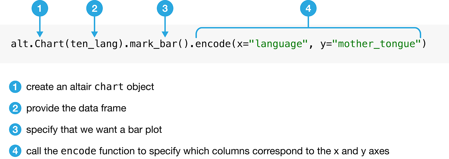
Fig. 1.8 Syntax for using altair to make a bar chart.

barplot_mother_tongue = (
  alt.Chart(ten_lang).mark_bar().encode(x="language", y="mother_tongue")
)

Fig. 1.9 Bar plot of the ten Aboriginal languages most often reported by Canadian residents as their mother tongue

1.11.2. Formatting altair charts

It is exciting that we can already visualize our data to help answer our question, but we are not done yet! We can (and should) do more to improve the interpretability of the data visualization that we created. For example, by default, Python uses the column names as the axis labels. Usually these column names do not have enough information about the variable in the column. We really should replace this default with a more informative label. For the example above, Python uses the column name mother_tongue as the label for the y axis, but most people will not know what that is. And even if they did, they will not know how we measured this variable, or the group of people on which the measurements were taken. An axis label that reads “Mother Tongue (Number of Canadian Residents)” would be much more informative. To make the code easier to read, we’re spreading it out over multiple lines just as we did in the previous section with pandas.

Adding additional labels to our visualizations that we create in altair is one common and easy way to improve and refine our data visualizations. We can add titles for the axes in the altair objects using alt.X and alt.Y with the title method to make the axes titles more informative (you will learn more about alt.X and alt.Y in Chapter 4). Again, since we are specifying words (e.g. "Mother Tongue (Number of Canadian Residents)") as arguments to the title method, we surround them with quotation marks. We can do many other modifications to format the plot further, and we will explore these in Chapter 4.

barplot_mother_tongue = alt.Chart(ten_lang).mark_bar().encode(
    x=alt.X("language").title("Language"),
    y=alt.Y("mother_tongue").title("Mother Tongue (Number of Canadian Residents)")
)

Fig. 1.10 Bar plot of the ten Aboriginal languages most often reported by Canadian residents as their mother tongue with x and y labels. Note that this visualization is not done yet; there are still improvements to be made.

The result is shown in Fig. 1.10. This is already quite an improvement! Let’s tackle the next major issue with the visualization in Fig. 1.10: the vertical x axis labels, which are currently making it difficult to read the different language names. One solution is to rotate the plot such that the bars are horizontal rather than vertical. To accomplish this, we will swap the x and y coordinate axes:

barplot_mother_tongue_axis = alt.Chart(ten_lang).mark_bar().encode(
    x=alt.X("mother_tongue").title("Mother Tongue (Number of Canadian Residents)"),
    y=alt.Y("language").title("Language")
)

Fig. 1.11 Horizontal bar plot of the ten Aboriginal languages most often reported by Canadian residents as their mother tongue. There are no more serious issues with this visualization, but it could be refined further.

Another big step forward, as shown in Fig. 1.11! There are no more serious issues with the visualization. Now comes time to refine the visualization to make it even more well-suited to answering the question we asked earlier in this chapter. For example, the visualization could be made more transparent by organizing the bars according to the number of Canadian residents reporting each language, rather than in alphabetical order. We can reorder the bars using the sort method, which orders a variable (here language) based on the values of the variable(mother_tongue) on the x-axis.

ordered_barplot_mother_tongue = alt.Chart(ten_lang).mark_bar().encode(
    x=alt.X("mother_tongue").title("Mother Tongue (Number of Canadian Residents)"),
    y=alt.Y("language").sort("x").title("Language")
)

Fig. 1.12 Bar plot of the ten Aboriginal languages most often reported by Canadian residents as their mother tongue with bars reordered.

Fig. 1.12 provides a very clear and well-organized answer to our original question; we can see what the ten most often reported Aboriginal languages were, according to the 2016 Canadian census, and how many people speak each of them. For instance, we can see that the Aboriginal language most often reported was Cree n.o.s. with over 60,000 Canadian residents reporting it as their mother tongue.

Note

“n.o.s.” means “not otherwise specified”, so Cree n.o.s. refers to individuals who reported Cree as their mother tongue. In this data set, the Cree languages include the following categories: Cree n.o.s., Swampy Cree, Plains Cree, Woods Cree, and a ‘Cree not included elsewhere’ category (which includes Moose Cree, Northern East Cree and Southern East Cree) [Statistics Canada, 2016].

1.11.3. Putting it all together

In the block of code below, we put everything from this chapter together, with a few modifications. In particular, we have combined all of our steps into one expression split across multiple lines using the left and right parenthesis symbols ( and ). We have also provided comments next to many of the lines of code below using the hash symbol #. When Python sees a # sign, it will ignore all of the text that comes after the symbol on that line. So you can use comments to explain lines of code for others, and perhaps more importantly, your future self! It’s good practice to get in the habit of commenting your code to improve its readability.

This exercise demonstrates the power of Python. In relatively few lines of code, we performed an entire data science workflow with a highly effective data visualization! We asked a question, loaded the data into Python, wrangled the data (using [], loc[], sort_values, and head) and created a data visualization to help answer our question. In this chapter, you got a quick taste of the data science workflow; continue on with the next few chapters to learn each of these steps in much more detail!

# load the data set
can_lang = pd.read_csv("data/can_lang.csv")

# obtain the 10 most common Aboriginal languages
ten_lang = (
    can_lang.loc[can_lang["category"] == "Aboriginal languages", ["language", "mother_tongue"]]
    .sort_values(by="mother_tongue", ascending=False)
    .head(10)
)

# create the visualization
ten_lang_plot = alt.Chart(ten_lang).mark_bar().encode(
    x=alt.X("mother_tongue").title("Mother Tongue (Number of Canadian Residents)"),
    y=alt.Y("language").sort("x").title("Language")
)

Fig. 1.13 Bar plot of the ten Aboriginal languages most often reported by Canadian residents as their mother tongue

1.12. Accessing documentation

There are many Python functions in the pandas package (and beyond!), and nobody can be expected to remember what every one of them does or all of the arguments we have to give them. Fortunately, Python provides the help function, which provides an easy way to pull up the documentation for most functions quickly. To use the help function to access the documentation, you just put the name of the function you are curious about as an argument inside the help function. For example, if you had forgotten what the pd.read_csv function did or exactly what arguments to pass in, you could run the following code:

help(pd.read_csv)

Fig. 1.14 shows the documentation that will pop up, including a high-level description of the function, its arguments, a description of each, and more. Note that you may find some of the text in the documentation a bit too technical right now. Fear not: as you work through this book, many of these terms will be introduced to you, and slowly but surely you will become more adept at understanding and navigating documentation like that shown in Fig. 1.14. But do keep in mind that the documentation is not written to teach you about a function; it is just there as a reference to remind you about the different arguments and usage of functions that you have already learned about elsewhere.

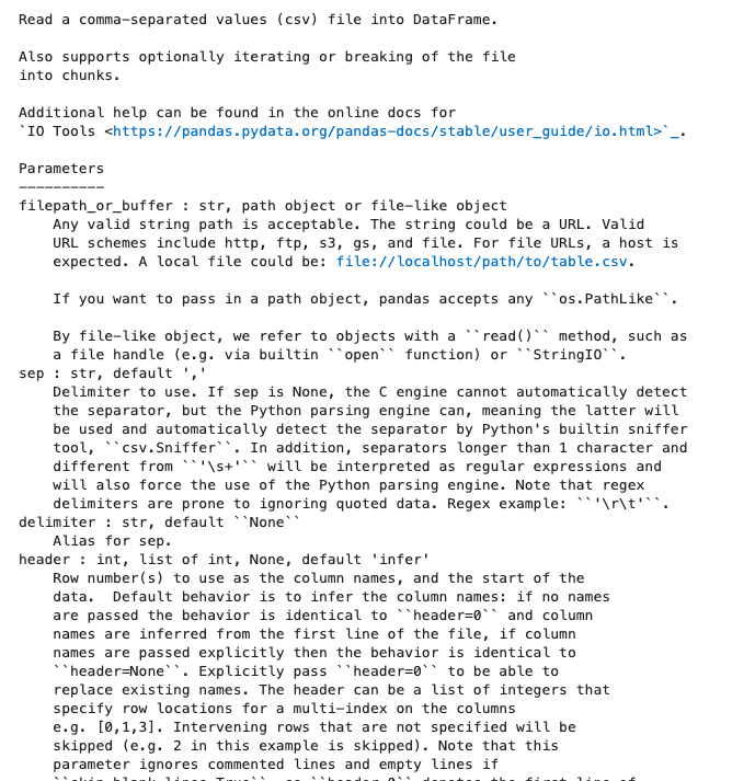
Fig. 1.14 The documentation for the read_csv function including a high-level description, a list of arguments and their meanings, and more.

If you are working in a Jupyter Lab environment, there are some conveniences that will help you lookup function names and access the documentation. First, rather than help, you can use the more concise ? character. So for example, to read the documentation for the pd.read_csv function, you can run the following code:

?pd.read_csv

You can also type the first characters of the function you want to use, and then press Tab to bring up small menu that shows you all the available functions that starts with those characters. This is helpful both for remembering function names and to prevent typos.

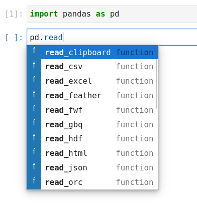
Fig. 1.15 The suggestions that are shown after typing pd.read and pressing Tab.

To get more info on the function you want to use, you can type out the full name and then hold Shift while pressing Tab to bring up a help dialogue including the same information as when using help().

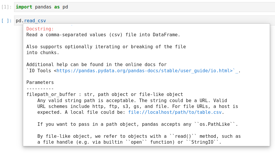
Fig. 1.16 The help dialog that is shown after typing pd.read_csv and then pressing Shift + Tab.

Finally, it can be helpful to have this help dialog open at all times, especially when you start out learning about programming and data science. You can achieve this by clicking on the Help text in the menu bar at the top and then selecting Show Contextual Help.

1.13. Exercises

Practice exercises for the material covered in this chapter can be found in the accompanying worksheets repository in the “Python and Pandas” row. You can launch an interactive version of the worksheet in your browser by clicking the “launch binder” button. You can also preview a non-interactive version of the worksheet by clicking “view worksheet.” If you instead decide to download the worksheet and run it on your own machine, make sure to follow the instructions for computer setup found in Chapter 13. This will ensure that the automated feedback and guidance that the worksheets provide will function as intended.

1.14. References

GvR01

Nick Coghlan Guido van Rossum, Barry Warsaw. PEP 8 – Style Guide for Python Code. 2001. URL: https://peps.python.org/pep-0008/.

LP15

Jeffrey Leek and Roger Peng. What is the question? Science, 347(6228):1314–1315, 2015.

PM15

Roger D Peng and Elizabeth Matsui. The Art of Data Science: A Guide for Anyone Who Works with Data. Skybrude Consulting, LLC, 2015. URL: https://bookdown.org/rdpeng/artofdatascience/.

Tim20

Tiffany Timbers. canlang: Canadian Census language data. 2020. R package version 0.0.9. URL: https://ttimbers.github.io/canlang/.

Wal17

Nick Walker. Mapping indigenous languages in Canada. Canadian Geographic, 2017. URL: https://www.canadiangeographic.ca/article/mapping-indigenous-languages-canada (visited on 2021-05-27).

Wil18

Kory Wilson. Pulling Together: Foundations Guide. BCcampus, 2018. URL: https://opentextbc.ca/indigenizationfoundations/ (visited on 2021-05-27).

StatisticsCanada16a

Statistics Canada. Population census. 2016. URL: https://www12.statcan.gc.ca/census-recensement/2016/dp-pd/index-eng.cfm.

StatisticsCanada16b

Statistics Canada. The Aboriginal languages of First Nations people, Métis and Inuit. 2016. URL: https://www12.statcan.gc.ca/census-recensement/2016/as-sa/98-200-x/2016022/98-200-x2016022-eng.cfm.

StatisticsCanada18

Statistics Canada. The evolution of language populations in Canada, by mother tongue, from 1901 to 2016. 2018. URL: https://www150.statcan.gc.ca/n1/pub/11-630-x/11-630-x2018001-eng.htm (visited on 2021-05-27).

ThePDTeam20

The Pandas Development Team. pandas-dev/pandas: Pandas. February 2020. URL: https://doi.org/10.5281/zenodo.3509134, doi:10.5281/zenodo.3509134.

TruthaRCoCanada12

Truth and Reconciliation Commission of Canada. They Came for the Children: Canada, Aboriginal Peoples, and the Residential Schools. Public Works & Government Services Canada, 2012.

TruthaRCoCanada15

Truth and Reconciliation Commission of Canada. Calls to Action. 2015. URL: https://www2.gov.bc.ca/assets/gov/british-columbians-our-governments/indigenous-people/aboriginal-peoples-documents/calls_to_action_english2.pdf.

WesMcKinney10

Wes McKinney. Data Structures for Statistical Computing in Python. In Stéfan van der Walt and Jarrod Millman, editors, Proceedings of the 9th Python in Science Conference, 56 – 61. 2010. doi:10.25080/Majora-92bf1922-00a.