3. Cleaning and wrangling data

3.1. Overview

This chapter is centered around defining tidy data—a data format that is suitable for analysis—and the tools needed to transform raw data into this format. This will be presented in the context of a real-world data science application, providing more practice working through a whole case study.

3.2. Chapter learning objectives

By the end of the chapter, readers will be able to do the following:

• Define the term “tidy data”.

• Discuss the advantages of storing data in a tidy data format.

• Define what series and data frames are in Python, and describe how they relate to each other.

• Describe the common types of data in Python and their uses.

• Use the following functions for their intended data wrangling tasks:

  • melt

  • pivot

  • reset_index

  • str.split

  • agg

  • assign and regular column assignment

  • groupby

  • merge

• Use the following operators for their intended data wrangling tasks:

  • ==, !=, <, >, <=, and >=

  • isin

  • & and |

  • [], loc[], and iloc[]

3.3. Data frames and series

In Chapters 1 and 2, data frames were the focus: we learned how to import data into Python as a data frame, and perform basic operations on data frames in Python. In the remainder of this book, this pattern continues. The vast majority of tools we use will require that data are represented as a pandas data frame in Python. Therefore, in this section, we will dig more deeply into what data frames are and how they are represented in Python. This knowledge will be helpful in effectively utilizing these objects in our data analyses.

3.3.1. What is a data frame?

A data frame is a table-like structure for storing data in Python. Data frames are important to learn about because most data that you will encounter in practice can be naturally stored as a table. In order to define data frames precisely, we need to introduce a few technical terms:

• variable: a characteristic, number, or quantity that can be measured.

• observation: all of the measurements for a given entity.

• value: a single measurement of a single variable for a given entity.

Given these definitions, a data frame is a tabular data structure in Python that is designed to store observations, variables, and their values. Most commonly, each column in a data frame corresponds to a variable, and each row corresponds to an observation. For example, Fig. 3.1 displays a data set of city populations. Here, the variables are “region, year, population”; each of these are properties that can be collected or measured. The first observation is “Toronto, 2016, 2235145”; these are the values that the three variables take for the first entity in the data set. There are 13 entities in the data set in total, corresponding to the 13 rows in Fig. 3.1.

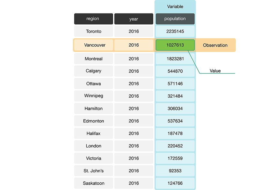
Fig. 3.1 A data frame storing data regarding the population of various regions in Canada. In this example data frame, the row that corresponds to the observation for the city of Vancouver is colored yellow, and the column that corresponds to the population variable is colored blue.

3.3.2. What is a series?

In Python, pandas series are are objects that can contain one or more elements (like a list). They are a single column, are ordered, can be indexed, and can contain any data type. The pandas package uses Series objects to represent the columns in a data frame. Series can contain a mix of data types, but it is good practice to only include a single type in a series because all observations of one variable should be the same type. Python has several different basic data types, as shown in Table 3.1. You can create a pandas series using the pd.Series() function. For example, to create the series region as shown in Fig. 3.2, you can write the following.

import pandas as pd

region = pd.Series(["Toronto", "Montreal", "Vancouver", "Calgary", "Ottawa"])
region

0      Toronto
1     Montreal
2    Vancouver
3      Calgary
4       Ottawa
dtype: object

Fig. 3.2 Example of a pandas series whose type is string.

Table 3.1 Basic data types in Python

Data type	Abbreviation	Description	Example
integer	int	positive/negative/zero whole numbers	42
floating point number	float	real number in decimal form	3.14159
boolean	bool	true or false	True
string	str	text	"Hello World"
none	NoneType	represents no value	None

It is important in Python to make sure you represent your data with the correct type. Many of the pandas functions we use in this book treat the various data types differently. You should use int and float types to represent numbers and perform arithmetic. The int type is for integers that have no decimal point, while the float type is for numbers that have a decimal point. The bool type are boolean variables that can only take on one of two values: True or False. The string type is used to represent data that should be thought of as “text”, such as words, names, paths, URLs, and more. A NoneType is a special type in Python that is used to indicate no value; this can occur, for example, when you have missing data. There are other basic data types in Python, but we will generally not use these in this textbook.

3.3.3. What does this have to do with data frames?

A data frame is really just a collection of series that are stuck together, where each series corresponds to one column and all must have the same length. But not all columns in a data frame need to be of the same type. Fig. 3.3 shows a data frame where the columns are series of different types. But each element within one column should usually be the same type, since the values for a single variable are usually all of the same type. For example, if the variable is the name of a city, that name should be a string, whereas if the variable is a year, that should be an integer. So even though series let you put different types in them, it is most common (and good practice!) to have just one type per column.

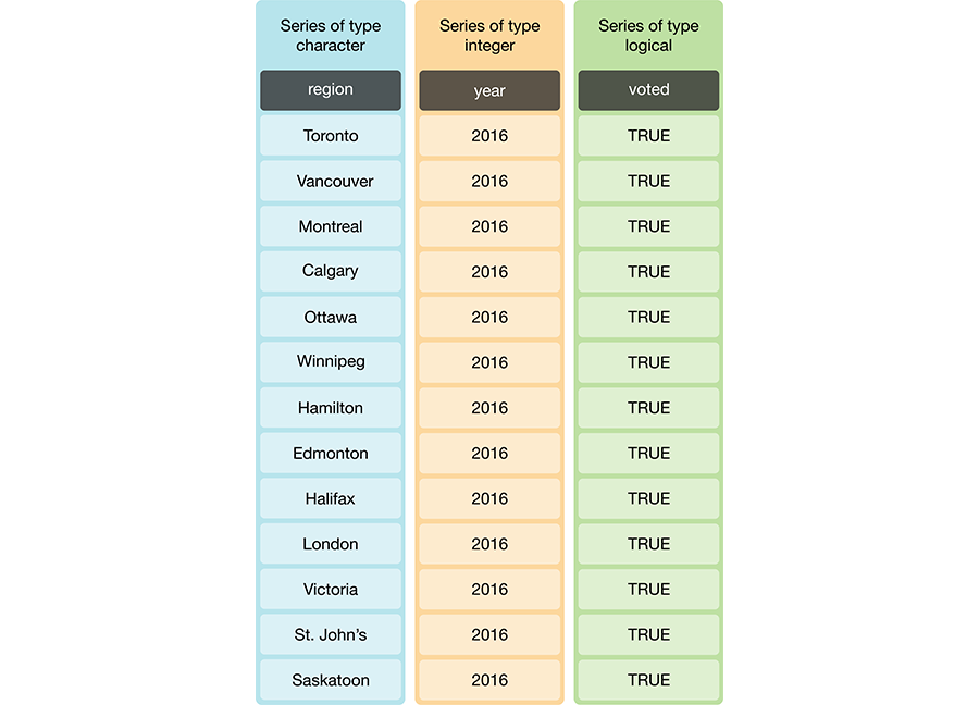
Fig. 3.3 Data frame and series types.

Note

You can use the function type on a data object. For example we can check the class of the Canadian languages data set, can_lang, we worked with in the previous chapters and we see it is a pandas.core.frame.DataFrame.

can_lang = pd.read_csv("data/can_lang.csv")
type(can_lang)

pandas.core.frame.DataFrame

3.3.4. Data structures in Python

The Series and DataFrame types are data structures in Python, which are core to most data analyses. The functions from pandas that we use often give us back a DataFrame or a Series depending on the operation. Because Series are essentially simple DataFrames, we will refer to both DataFrames and Series as “data frames” in the text. There are other types that represent data structures in Python. We summarize the most common ones in Table 3.2.

Table 3.2 Basic data structures in Python

Data Structure	Description
list	An ordered collection of values that can store multiple data types at once.
dict	A labeled data structure where keys are paired with values
Series	An ordered collection of values with labels that can store multiple data types at once.
DataFrame	A labeled data structure with Series columns of potentially different types.

A list is an ordered collection of values. To create a list, we put the contents of the list in between square brackets [], where each item of the list is separated by a comma. A list can contain values of different types. The example below contains six str entries.

cities = ["Toronto", "Vancouver", "Montreal", "Calgary", "Ottawa", "Winnipeg"]
cities

['Toronto', 'Vancouver', 'Montreal', 'Calgary', 'Ottawa', 'Winnipeg']

A list can directly be converted to a pandas Series.

cities_series = pd.Series(cities)
cities_series

0      Toronto
1    Vancouver
2     Montreal
3      Calgary
4       Ottawa
5     Winnipeg
dtype: object

A dict, or dictionary, contains pairs of “keys” and “values.” You use a key to look up its corresponding value. Dictionaries are created using curly brackets {}. Each entry starts with the key on the left, followed by a colon symbol :, and then the value. A dictionary can have multiple key-value pairs, each separted by a comma. Keys can take a wide variety of types (int and str are commonly used), and values can take any type; the key-value pairs in a dictionary can all be of different types, too. In the example below, we create a dictionary that has two keys: "cities" and "population". The values associated with each are lists.

population_in_2016 = {
  "cities": ["Toronto", "Vancouver", "Montreal", "Calgary", "Ottawa", "Winnipeg"],
  "population": [2235145, 1027613, 1823281, 544870, 571146, 321484]
}
population_in_2016

{'cities': ['Toronto',
  'Vancouver',
  'Montreal',
  'Calgary',
  'Ottawa',
  'Winnipeg'],
 'population': [2235145, 1027613, 1823281, 544870, 571146, 321484]}

A dictionary can be converted to a data frame. Keys become the column names, and the values become the entries in those columns. Dictionaries on their own are quite simple objects; it is preferable to work with a data frame because then we have access to the built-in functionality in pandas (e.g. loc[], [], and many functions that we will discuss in the upcoming sections)!

population_in_2016_df = pd.DataFrame(population_in_2016)
population_in_2016_df

	cities	population
0	Toronto	2235145
1	Vancouver	1027613
2	Montreal	1823281
3	Calgary	544870
4	Ottawa	571146
5	Winnipeg	321484

Of course, there is no need to name the dictionary separately before passing it to pd.DataFrame; we can instead construct the dictionary right inside the call. This is often the most convenient way to create a new data frame.

population_in_2016_df = pd.DataFrame({
  "cities": ["Toronto", "Vancouver", "Montreal", "Calgary", "Ottawa", "Winnipeg"],
  "population": [2235145, 1027613, 1823281, 544870, 571146, 321484]
})
population_in_2016_df

	cities	population
0	Toronto	2235145
1	Vancouver	1027613
2	Montreal	1823281
3	Calgary	544870
4	Ottawa	571146
5	Winnipeg	321484

3.4. Tidy data

There are many ways a tabular data set can be organized. The data frames we have looked at so far have all been using the tidy data format of organization. This chapter will focus on introducing the tidy data format and how to make your raw (and likely messy) data tidy. A tidy data frame satisfies the following three criteria [Wickham, 2014]:

• each row is a single observation,

• each column is a single variable, and

• each value is a single cell (i.e., its entry in the data frame is not shared with another value).

Fig. 3.4 demonstrates a tidy data set that satisfies these three criteria.

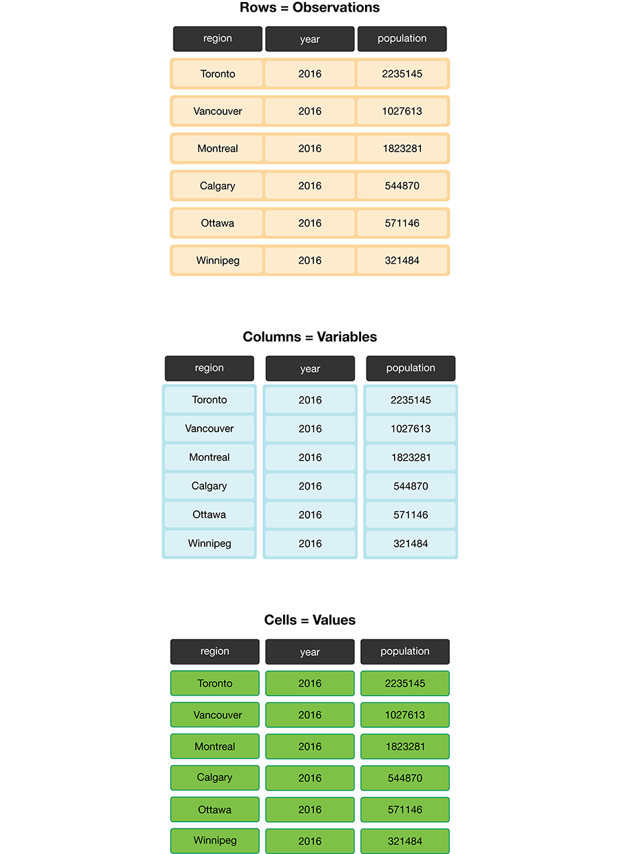
Fig. 3.4 Tidy data satisfies three criteria.

There are many good reasons for making sure your data are tidy as a first step in your analysis. The most important is that it is a single, consistent format that nearly every function in the pandas recognizes. No matter what the variables and observations in your data represent, as long as the data frame is tidy, you can manipulate it, plot it, and analyze it using the same tools. If your data is not tidy, you will have to write special bespoke code in your analysis that will not only be error-prone, but hard for others to understand. Beyond making your analysis more accessible to others and less error-prone, tidy data is also typically easy for humans to interpret. Given these benefits, it is well worth spending the time to get your data into a tidy format upfront. Fortunately, there are many well-designed pandas data cleaning/wrangling tools to help you easily tidy your data. Let’s explore them below!

Note

Is there only one shape for tidy data for a given data set? Not necessarily! It depends on the statistical question you are asking and what the variables are for that question. For tidy data, each variable should be its own column. So, just as it’s essential to match your statistical question with the appropriate data analysis tool, it’s important to match your statistical question with the appropriate variables and ensure they are represented as individual columns to make the data tidy.

3.4.1. Tidying up: going from wide to long using melt

One task that is commonly performed to get data into a tidy format is to combine values that are stored in separate columns, but are really part of the same variable, into one. Data is often stored this way because this format is sometimes more intuitive for human readability and understanding, and humans create data sets. In Fig. 3.5, the table on the left is in an untidy, “wide” format because the year values (2006, 2011, 2016) are stored as column names. And as a consequence, the values for population for the various cities over these years are also split across several columns.

For humans, this table is easy to read, which is why you will often find data stored in this wide format. However, this format is difficult to work with when performing data visualization or statistical analysis using Python. For example, if we wanted to find the latest year it would be challenging because the year values are stored as column names instead of as values in a single column. So before we could apply a function to find the latest year (for example, by using max), we would have to first extract the column names to get them as a list and then apply a function to extract the latest year. The problem only gets worse if you would like to find the value for the population for a given region for the latest year. Both of these tasks are greatly simplified once the data is tidied.

Another problem with data in this format is that we don’t know what the numbers under each year actually represent. Do those numbers represent population size? Land area? It’s not clear. To solve both of these problems, we can reshape this data set to a tidy data format by creating a column called “year” and a column called “population.” This transformation—which makes the data “longer”—is shown as the right table in Fig. 3.5. Note that the number of entries in our data frame can change in this transformation. The “untidy” data has 5 rows and 3 columns for a total of 15 entries, whereas the “tidy” data on the right has 15 rows and 2 columns for a total of 30 entries.

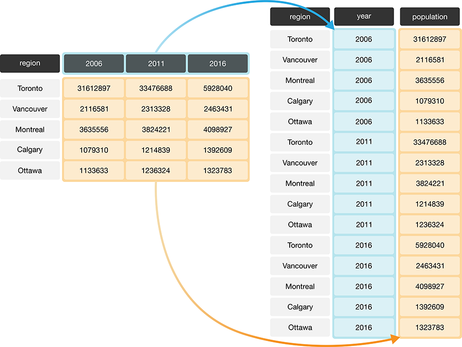
Fig. 3.5 Melting data from a wide to long data format.

We can achieve this effect in Python using the melt function from the pandas package. The melt function combines columns, and is usually used during tidying data when we need to make the data frame longer and narrower. To learn how to use melt, we will work through an example with the region_lang_top5_cities_wide.csv data set. This data set contains the counts of how many Canadians cited each language as their mother tongue for five major Canadian cities (Toronto, Montréal, Vancouver, Calgary, and Edmonton) from the 2016 Canadian census. To get started, we will use pd.read_csv to load the (untidy) data.

lang_wide = pd.read_csv("data/region_lang_top5_cities_wide.csv")
lang_wide

	category	language	Toronto	Montréal	Vancouver	Calgary	Edmonton
0	Aboriginal languages	Aboriginal languages, n.o.s.	80	30	70	20	25
1	Non-Official & Non-Aboriginal languages	Afrikaans	985	90	1435	960	575
2	Non-Official & Non-Aboriginal languages	Afro-Asiatic languages, n.i.e.	360	240	45	45	65
3	Non-Official & Non-Aboriginal languages	Akan (Twi)	8485	1015	400	705	885
4	Non-Official & Non-Aboriginal languages	Albanian	13260	2450	1090	1365	770
...	...	...	...	...	...	...	...
209	Non-Official & Non-Aboriginal languages	Wolof	165	2440	30	120	130
210	Aboriginal languages	Woods Cree	5	0	20	10	155
211	Non-Official & Non-Aboriginal languages	Wu (Shanghainese)	5290	1025	4330	380	235
212	Non-Official & Non-Aboriginal languages	Yiddish	3355	8960	220	80	55
213	Non-Official & Non-Aboriginal languages	Yoruba	3380	210	190	1430	700

214 rows × 7 columns

What is wrong with the untidy format above? The table on the left in Fig. 3.6 represents the data in the “wide” (messy) format. From a data analysis perspective, this format is not ideal because the values of the variable region (Toronto, Montréal, Vancouver, Calgary, and Edmonton) are stored as column names. Thus they are not easily accessible to the data analysis functions we will apply to our data set. Additionally, the mother tongue variable values are spread across multiple columns, which will prevent us from doing any desired visualization or statistical tasks until we combine them into one column. For instance, suppose we want to know the languages with the highest number of Canadians reporting it as their mother tongue among all five regions. This question would be tough to answer with the data in its current format. We could find the answer with the data in this format, though it would be much easier to answer if we tidy our data first. If mother tongue were instead stored as one column, as shown in the tidy data on the right in Fig. 3.6, we could simply use one line of code (df["mother_tongue"].max()) to get the maximum value.

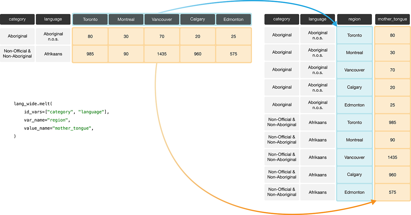
Fig. 3.6 Going from wide to long with the melt function.

Fig. 3.7 details the arguments that we need to specify in the melt function to accomplish this data transformation.

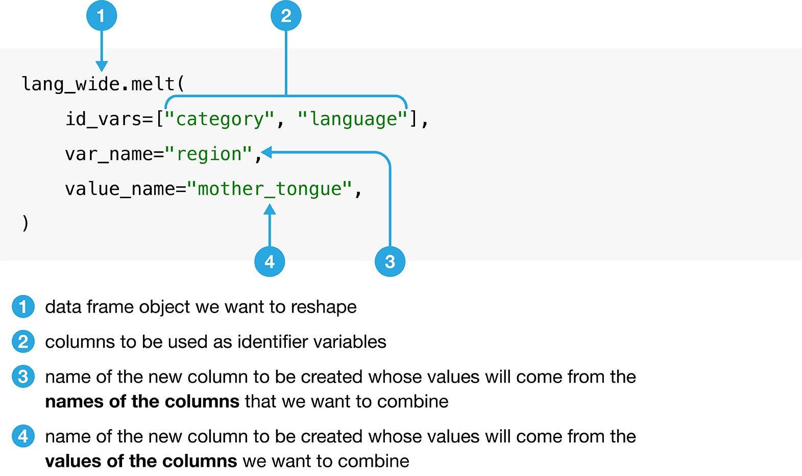
Fig. 3.7 Syntax for the melt function.

We use melt to combine the Toronto, Montréal, Vancouver, Calgary, and Edmonton columns into a single column called region, and create a column called mother_tongue that contains the count of how many Canadians report each language as their mother tongue for each metropolitan area

lang_mother_tidy = lang_wide.melt(
    id_vars=["category", "language"],
    var_name="region",
    value_name="mother_tongue",
)
lang_mother_tidy

	category	language	region	mother_tongue
0	Aboriginal languages	Aboriginal languages, n.o.s.	Toronto	80
1	Non-Official & Non-Aboriginal languages	Afrikaans	Toronto	985
2	Non-Official & Non-Aboriginal languages	Afro-Asiatic languages, n.i.e.	Toronto	360
3	Non-Official & Non-Aboriginal languages	Akan (Twi)	Toronto	8485
4	Non-Official & Non-Aboriginal languages	Albanian	Toronto	13260
...	...	...	...	...
1065	Non-Official & Non-Aboriginal languages	Wolof	Edmonton	130
1066	Aboriginal languages	Woods Cree	Edmonton	155
1067	Non-Official & Non-Aboriginal languages	Wu (Shanghainese)	Edmonton	235
1068	Non-Official & Non-Aboriginal languages	Yiddish	Edmonton	55
1069	Non-Official & Non-Aboriginal languages	Yoruba	Edmonton	700

1070 rows × 4 columns

Note

In the code above, the call to the melt function is split across several lines. Recall from Chapter 1 that this is allowed in certain cases. For example, when calling a function as above, the input arguments are between parentheses () and Python knows to keep reading on the next line. Each line ends with a comma , making it easier to read. Splitting long lines like this across multiple lines is encouraged as it helps significantly with code readability. Generally speaking, you should limit each line of code to about 80 characters.

The data above is now tidy because all three criteria for tidy data have now been met:

1. All the variables (category, language, region and mother_tongue) are now their own columns in the data frame.

2. Each observation, i.e., each category, language, region, and count of Canadians where that language is the mother tongue, are in a single row.

3. Each value is a single cell, i.e., its row, column position in the data frame is not shared with another value.

3.4.2. Tidying up: going from long to wide using pivot

Suppose we have observations spread across multiple rows rather than in a single row. For example, in Fig. 3.8, the table on the left is in an untidy, long format because the count column contains three variables (population, commuter, and incorporated count) and information about each observation (here, population, commuter, and incorporated counts for a region) is split across three rows. Remember: one of the criteria for tidy data is that each observation must be in a single row.

Using data in this format—where two or more variables are mixed together in a single column—makes it harder to apply many usual pandas functions. For example, finding the maximum number of commuters would require an additional step of filtering for the commuter values before the maximum can be computed. In comparison, if the data were tidy, all we would have to do is compute the maximum value for the commuter column. To reshape this untidy data set to a tidy (and in this case, wider) format, we need to create columns called “population”, “commuters”, and “incorporated.” This is illustrated in the right table of Fig. 3.8.

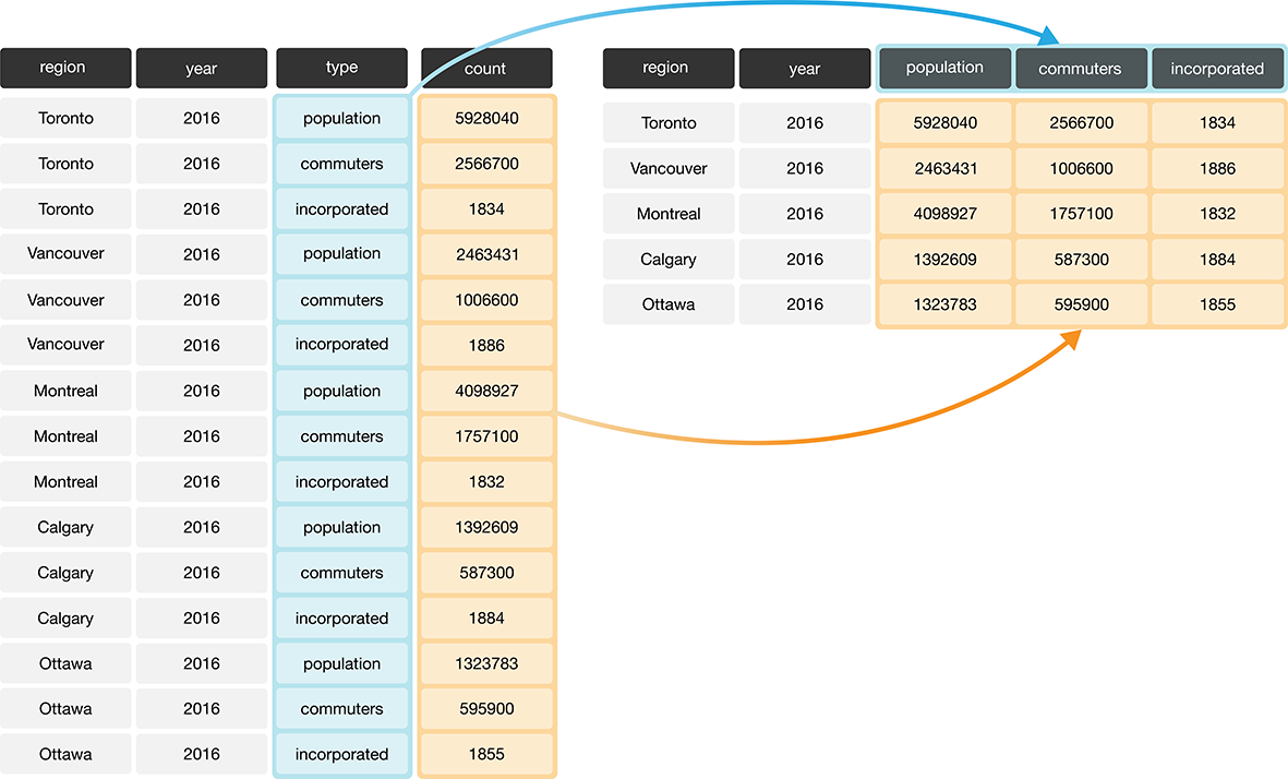
Fig. 3.8 Going from long to wide data.

To tidy this type of data in Python, we can use the pivot function. The pivot function generally increases the number of columns (widens) and decreases the number of rows in a data set. To learn how to use pivot, we will work through an example with the region_lang_top5_cities_long.csv data set. This data set contains the number of Canadians reporting the primary language at home and work for five major cities (Toronto, Montréal, Vancouver, Calgary, and Edmonton).

lang_long = pd.read_csv("data/region_lang_top5_cities_long.csv")
lang_long

	region	category	language	type	count
0	Montréal	Aboriginal languages	Aboriginal languages, n.o.s.	most_at_home	15
1	Montréal	Aboriginal languages	Aboriginal languages, n.o.s.	most_at_work	0
2	Toronto	Aboriginal languages	Aboriginal languages, n.o.s.	most_at_home	50
3	Toronto	Aboriginal languages	Aboriginal languages, n.o.s.	most_at_work	0
4	Calgary	Aboriginal languages	Aboriginal languages, n.o.s.	most_at_home	5
...	...	...	...	...	...
2135	Calgary	Non-Official & Non-Aboriginal languages	Yoruba	most_at_work	0
2136	Edmonton	Non-Official & Non-Aboriginal languages	Yoruba	most_at_home	280
2137	Edmonton	Non-Official & Non-Aboriginal languages	Yoruba	most_at_work	0
2138	Vancouver	Non-Official & Non-Aboriginal languages	Yoruba	most_at_home	40
2139	Vancouver	Non-Official & Non-Aboriginal languages	Yoruba	most_at_work	0

2140 rows × 5 columns

What makes the data set shown above untidy? In this example, each observation is a language in a region. However, each observation is split across multiple rows: one where the count for most_at_home is recorded, and the other where the count for most_at_work is recorded. Suppose the goal with this data was to visualize the relationship between the number of Canadians reporting their primary language at home and work. Doing that would be difficult with this data in its current form, since these two variables are stored in the same column. Fig. 3.9 shows how this data will be tidied using the pivot function.

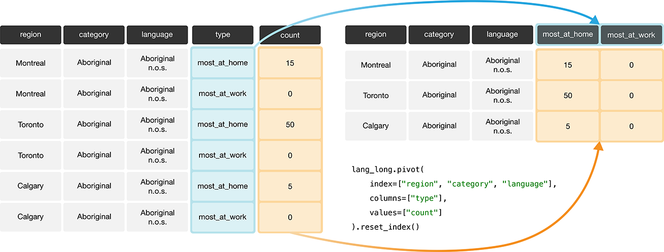
Fig. 3.9 Going from long to wide with the pivot function.

Fig. 3.10 details the arguments that we need to specify in the pivot function.

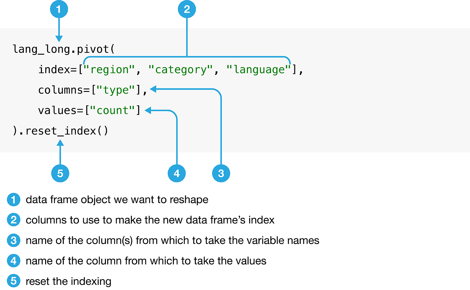
Fig. 3.10 Syntax for the pivot function.

We will apply the function as detailed in Fig. 3.10, and then rename the columns.

lang_home_tidy = lang_long.pivot(
    index=["region", "category", "language"],
    columns=["type"],
    values=["count"]
).reset_index()

lang_home_tidy.columns = [
    "region",
    "category",
    "language",
    "most_at_home",
    "most_at_work",
]
lang_home_tidy

	region	category	language	most_at_home	most_at_work
0	Calgary	Aboriginal languages	Aboriginal languages, n.o.s.	5	0
1	Calgary	Aboriginal languages	Algonquian languages, n.i.e.	0	0
2	Calgary	Aboriginal languages	Algonquin	0	0
3	Calgary	Aboriginal languages	Athabaskan languages, n.i.e.	0	0
4	Calgary	Aboriginal languages	Atikamekw	0	0
...	...	...	...	...	...
1065	Vancouver	Non-Official & Non-Aboriginal languages	Wu (Shanghainese)	2495	45
1066	Vancouver	Non-Official & Non-Aboriginal languages	Yiddish	10	0
1067	Vancouver	Non-Official & Non-Aboriginal languages	Yoruba	40	0
1068	Vancouver	Official languages	English	1622735	1330555
1069	Vancouver	Official languages	French	8630	3245

1070 rows × 5 columns

In the first step, note that we added a call to reset_index. When pivot is called with multiple column names passed to the index, those entries become the “name” of each row that would be used when you filter rows with [] or loc rather than just simple numbers. This can be confusing… What reset_index does is sets us back with the usual expected behaviour where each row is “named” with an integer. This is a subtle point, but the main take-away is that when you call pivot, it is a good idea to call reset_index afterwards.

The second operation we applied is to rename the columns. When we perform the pivot operation, it keeps the original column name "count" and adds the "type" as a second column name. Having two names for a column can be confusing! So we rename giving each column only one name.

We can print out some useful information about our data frame using the info function. In the first row it tells us the type of lang_home_tidy (it is a pandas DataFrame). The second row tells us how many rows there are: 1070, and to index those rows, you can use numbers between 0 and 1069 (remember that Python starts counting at 0!). Next, there is a print out about the data colums. Here there are 5 columns total. The little table it prints out tells you the name of each column, the number of non-null values (e.g. the number of entries that are not missing values), and the type of the entries. Finally the last two rows summarize the types of each column and how much memory the data frame is using on your computer.

lang_home_tidy.info()

<class 'pandas.core.frame.DataFrame'>
RangeIndex: 1070 entries, 0 to 1069
Data columns (total 5 columns):
 #   Column        Non-Null Count  Dtype 
---  ------        --------------  ----- 
 0   region        1070 non-null   object
 1   category      1070 non-null   object
 2   language      1070 non-null   object
 3   most_at_home  1070 non-null   int64 
 4   most_at_work  1070 non-null   int64 
dtypes: int64(2), object(3)
memory usage: 41.9+ KB

The data is now tidy! We can go through the three criteria again to check that this data is a tidy data set.

1. All the statistical variables are their own columns in the data frame (i.e., most_at_home, and most_at_work have been separated into their own columns in the data frame).

2. Each observation, (i.e., each language in a region) is in a single row.

3. Each value is a single cell (i.e., its row, column position in the data frame is not shared with another value).

You might notice that we have the same number of columns in the tidy data set as we did in the messy one. Therefore pivot didn’t really “widen” the data. This is just because the original type column only had two categories in it. If it had more than two, pivot would have created more columns, and we would see the data set “widen.”

3.4.3. Tidying up: using str.split to deal with multiple separators

Data are also not considered tidy when multiple values are stored in the same cell. The data set we show below is even messier than the ones we dealt with above: the Toronto, Montréal, Vancouver, Calgary, and Edmonton columns contain the number of Canadians reporting their primary language at home and work in one column separated by the separator (/). The column names are the values of a variable, and each value does not have its own cell! To turn this messy data into tidy data, we’ll have to fix these issues.

lang_messy = pd.read_csv("data/region_lang_top5_cities_messy.csv")
lang_messy

	category	language	Toronto	Montréal	Vancouver	Calgary	Edmonton
0	Aboriginal languages	Aboriginal languages, n.o.s.	50/0	15/0	15/0	5/0	10/0
1	Non-Official & Non-Aboriginal languages	Afrikaans	265/0	10/0	520/10	505/15	300/0
2	Non-Official & Non-Aboriginal languages	Afro-Asiatic languages, n.i.e.	185/10	65/0	10/0	15/0	20/0
3	Non-Official & Non-Aboriginal languages	Akan (Twi)	4045/20	440/0	125/10	330/0	445/0
4	Non-Official & Non-Aboriginal languages	Albanian	6380/215	1445/20	530/10	620/25	370/10
...	...	...	...	...	...	...	...
209	Non-Official & Non-Aboriginal languages	Wolof	75/0	770/0	5/0	65/0	90/10
210	Aboriginal languages	Woods Cree	0/10	0/0	5/0	0/0	20/0
211	Non-Official & Non-Aboriginal languages	Wu (Shanghainese)	3130/30	760/15	2495/45	210/0	120/0
212	Non-Official & Non-Aboriginal languages	Yiddish	350/20	6665/860	10/0	10/0	0/0
213	Non-Official & Non-Aboriginal languages	Yoruba	1080/10	45/0	40/0	350/0	280/0

214 rows × 7 columns

First we’ll use melt to create two columns, region and value, similar to what we did previously. The new region columns will contain the region names, and the new column value will be a temporary holding place for the data that we need to further separate, i.e., the number of Canadians reporting their primary language at home and work.

lang_messy_longer = lang_messy.melt(
    id_vars=["category", "language"],
    var_name="region",
    value_name="value",
)

lang_messy_longer

	category	language	region	value
0	Aboriginal languages	Aboriginal languages, n.o.s.	Toronto	50/0
1	Non-Official & Non-Aboriginal languages	Afrikaans	Toronto	265/0
2	Non-Official & Non-Aboriginal languages	Afro-Asiatic languages, n.i.e.	Toronto	185/10
3	Non-Official & Non-Aboriginal languages	Akan (Twi)	Toronto	4045/20
4	Non-Official & Non-Aboriginal languages	Albanian	Toronto	6380/215
...	...	...	...	...
1065	Non-Official & Non-Aboriginal languages	Wolof	Edmonton	90/10
1066	Aboriginal languages	Woods Cree	Edmonton	20/0
1067	Non-Official & Non-Aboriginal languages	Wu (Shanghainese)	Edmonton	120/0
1068	Non-Official & Non-Aboriginal languages	Yiddish	Edmonton	0/0
1069	Non-Official & Non-Aboriginal languages	Yoruba	Edmonton	280/0

1070 rows × 4 columns

Next we’ll split the value column into two columns. In basic Python, if we wanted to split the string "50/0" into two numbers ["50", "0"] we would use the split method on the string, and specify that the split should be made on the slash character "/".

"50/0".split("/")

['50', '0']

The pandas package provides similar functions that we can access by using the str method. So to split all of the entries for an entire column in a data frame, we will use the str.split method. The output of this method is a data frame with two columns: one containing only the counts of Canadians that speak each language most at home, and the other containing only the counts of Canadians that speak each language most at work for each region. We drop the no-longer-needed value column from the lang_messy_longer data frame, and then assign the two columns from str.split to two new columns. Fig. 3.11 outlines what we need to specify to use str.split.

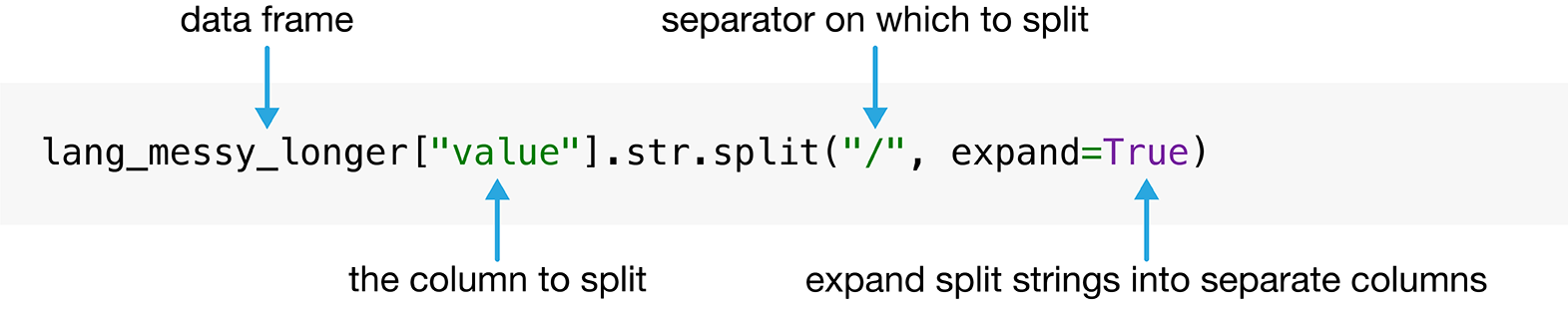
Fig. 3.11 Syntax for the str.split function.

tidy_lang = lang_messy_longer.drop(columns=["value"])
tidy_lang[["most_at_home", "most_at_work"]] = lang_messy_longer["value"].str.split("/", expand=True)
tidy_lang

	category	language	region	most_at_home	most_at_work
0	Aboriginal languages	Aboriginal languages, n.o.s.	Toronto	50	0
1	Non-Official & Non-Aboriginal languages	Afrikaans	Toronto	265	0
2	Non-Official & Non-Aboriginal languages	Afro-Asiatic languages, n.i.e.	Toronto	185	10
3	Non-Official & Non-Aboriginal languages	Akan (Twi)	Toronto	4045	20
4	Non-Official & Non-Aboriginal languages	Albanian	Toronto	6380	215
...	...	...	...	...	...
1065	Non-Official & Non-Aboriginal languages	Wolof	Edmonton	90	10
1066	Aboriginal languages	Woods Cree	Edmonton	20	0
1067	Non-Official & Non-Aboriginal languages	Wu (Shanghainese)	Edmonton	120	0
1068	Non-Official & Non-Aboriginal languages	Yiddish	Edmonton	0	0
1069	Non-Official & Non-Aboriginal languages	Yoruba	Edmonton	280	0

1070 rows × 5 columns

Is this data set now tidy? If we recall the three criteria for tidy data:

• each row is a single observation,

• each column is a single variable, and

• each value is a single cell.

We can see that this data now satisfies all three criteria, making it easier to analyze. But we aren’t done yet! Although we can’t see it in the data frame above, all of the variables are actually object data types. We can check this using the info method.

tidy_lang.info()

<class 'pandas.core.frame.DataFrame'>
RangeIndex: 1070 entries, 0 to 1069
Data columns (total 5 columns):
 #   Column        Non-Null Count  Dtype 
---  ------        --------------  ----- 
 0   category      1070 non-null   object
 1   language      1070 non-null   object
 2   region        1070 non-null   object
 3   most_at_home  1070 non-null   object
 4   most_at_work  1070 non-null   object
dtypes: object(5)
memory usage: 41.9+ KB

Object columns in pandas data frames are columns of strings or columns with mixed types. In the previous example in Section 3.4.2, the most_at_home and most_at_work variables were int64 (integer), which is a type of numeric data. This change is due to the separator (/) when we read in this messy data set. Python read these columns in as string types, and by default, str.split will return columns with the object data type.

It makes sense for region, category, and language to be stored as an object type since they hold categorical values. However, suppose we want to apply any functions that treat the most_at_home and most_at_work columns as a number (e.g., finding rows above a numeric threshold of a column). That won’t be possible if the variable is stored as an object. Fortunately, the astype method from pandas provides a natural way to fix problems like this: it will convert the column to a selected data type. In this case, we choose the int data type to indicate that these variables contain integer counts. Note that below we assign the new numerical series to the most_at_home and most_at_work columns in tidy_lang; we have seen this syntax before in Section 1.9, and we will discuss it in more depth later in this chapter in Section 3.11.

tidy_lang["most_at_home"] = tidy_lang["most_at_home"].astype("int")
tidy_lang["most_at_work"] = tidy_lang["most_at_work"].astype("int")
tidy_lang

	category	language	region	most_at_home	most_at_work
0	Aboriginal languages	Aboriginal languages, n.o.s.	Toronto	50	0
1	Non-Official & Non-Aboriginal languages	Afrikaans	Toronto	265	0
2	Non-Official & Non-Aboriginal languages	Afro-Asiatic languages, n.i.e.	Toronto	185	10
3	Non-Official & Non-Aboriginal languages	Akan (Twi)	Toronto	4045	20
4	Non-Official & Non-Aboriginal languages	Albanian	Toronto	6380	215
...	...	...	...	...	...
1065	Non-Official & Non-Aboriginal languages	Wolof	Edmonton	90	10
1066	Aboriginal languages	Woods Cree	Edmonton	20	0
1067	Non-Official & Non-Aboriginal languages	Wu (Shanghainese)	Edmonton	120	0
1068	Non-Official & Non-Aboriginal languages	Yiddish	Edmonton	0	0
1069	Non-Official & Non-Aboriginal languages	Yoruba	Edmonton	280	0

1070 rows × 5 columns

tidy_lang.info()

<class 'pandas.core.frame.DataFrame'>
RangeIndex: 1070 entries, 0 to 1069
Data columns (total 5 columns):
 #   Column        Non-Null Count  Dtype 
---  ------        --------------  ----- 
 0   category      1070 non-null   object
 1   language      1070 non-null   object
 2   region        1070 non-null   object
 3   most_at_home  1070 non-null   int64 
 4   most_at_work  1070 non-null   int64 
dtypes: int64(2), object(3)
memory usage: 41.9+ KB

Now we see most_at_home and most_at_work columns are of int64 data types, indicating they are integer data types (i.e., numbers)!

3.5. Using [] to extract rows or columns

Now that the tidy_lang data is indeed tidy, we can start manipulating it using the powerful suite of functions from the pandas. We will first revisit the [] from Chapter 1, which lets us obtain a subset of either the rows or the columns of a data frame. This section will highlight more advanced usage of the [] function, including an in-depth treatment of the variety of logical statements one can use in the [] to select subsets of rows.

3.5.1. Extracting columns by name

Recall that if we provide a list of column names, [] returns the subset of columns with those names as a data frame. Suppose we wanted to select the columns language, region, most_at_home and most_at_work from the tidy_lang data set. Using what we learned in Chapter 1, we can pass all of these column names into the square brackets.

tidy_lang[["language", "region", "most_at_home", "most_at_work"]]

	language	region	most_at_home	most_at_work
0	Aboriginal languages, n.o.s.	Toronto	50	0
1	Afrikaans	Toronto	265	0
2	Afro-Asiatic languages, n.i.e.	Toronto	185	10
3	Akan (Twi)	Toronto	4045	20
4	Albanian	Toronto	6380	215
...	...	...	...	...
1065	Wolof	Edmonton	90	10
1066	Woods Cree	Edmonton	20	0
1067	Wu (Shanghainese)	Edmonton	120	0
1068	Yiddish	Edmonton	0	0
1069	Yoruba	Edmonton	280	0

1070 rows × 4 columns

Likewise, if we pass a list containing a single column name, a data frame with this column will be returned.

tidy_lang[["language"]]

	language
0	Aboriginal languages, n.o.s.
1	Afrikaans
2	Afro-Asiatic languages, n.i.e.
3	Akan (Twi)
4	Albanian
...	...
1065	Wolof
1066	Woods Cree
1067	Wu (Shanghainese)
1068	Yiddish
1069	Yoruba

1070 rows × 1 columns

When we need to extract only a single column, we can also pass the column name as a string rather than a list. The returned data type will now be a series. Throughout this textbook, we will mostly extract single columns this way, but we will point out a few occasions where it is advantageous to extract single columns as data frames.

tidy_lang["language"]

0         Aboriginal languages, n.o.s.
1                            Afrikaans
2       Afro-Asiatic languages, n.i.e.
3                           Akan (Twi)
4                             Albanian
                     ...              
1065                             Wolof
1066                        Woods Cree
1067                 Wu (Shanghainese)
1068                           Yiddish
1069                            Yoruba
Name: language, Length: 1070, dtype: object

3.5.2. Extracting rows that have a certain value with ==

Suppose we are only interested in the subset of rows in tidy_lang corresponding to the official languages of Canada (English and French). We can extract these rows by using the equivalency operator (==) to compare the values of the category column with the value "Official languages". With these arguments, [] returns a data frame with all the columns of the input data frame but only the rows we asked for in the logical statement, i.e., those where the category column holds the value "Official languages". We name this data frame official_langs.

official_langs = tidy_lang[tidy_lang["category"] == "Official languages"]
official_langs

	category	language	region	most_at_home	most_at_work
54	Official languages	English	Toronto	3836770	3218725
59	Official languages	French	Toronto	29800	11940
268	Official languages	English	Montréal	620510	412120
273	Official languages	French	Montréal	2669195	1607550
482	Official languages	English	Vancouver	1622735	1330555
487	Official languages	French	Vancouver	8630	3245
696	Official languages	English	Calgary	1065070	844740
701	Official languages	French	Calgary	8630	2140
910	Official languages	English	Edmonton	1050410	792700
915	Official languages	French	Edmonton	10950	2520

3.5.3. Extracting rows that do not have a certain value with !=

What if we want all the other language categories in the data set except for those in the "Official languages" category? We can accomplish this with the != operator, which means “not equal to”. So if we want to find all the rows where the category does not equal "Official languages" we write the code below.

tidy_lang[tidy_lang["category"] != "Official languages"]

	category	language	region	most_at_home	most_at_work
0	Aboriginal languages	Aboriginal languages, n.o.s.	Toronto	50	0
1	Non-Official & Non-Aboriginal languages	Afrikaans	Toronto	265	0
2	Non-Official & Non-Aboriginal languages	Afro-Asiatic languages, n.i.e.	Toronto	185	10
3	Non-Official & Non-Aboriginal languages	Akan (Twi)	Toronto	4045	20
4	Non-Official & Non-Aboriginal languages	Albanian	Toronto	6380	215
...	...	...	...	...	...
1065	Non-Official & Non-Aboriginal languages	Wolof	Edmonton	90	10
1066	Aboriginal languages	Woods Cree	Edmonton	20	0
1067	Non-Official & Non-Aboriginal languages	Wu (Shanghainese)	Edmonton	120	0
1068	Non-Official & Non-Aboriginal languages	Yiddish	Edmonton	0	0
1069	Non-Official & Non-Aboriginal languages	Yoruba	Edmonton	280	0

1060 rows × 5 columns

3.5.4. Extracting rows satisfying multiple conditions using &

Suppose now we want to look at only the rows for the French language in Montréal. To do this, we need to filter the data set to find rows that satisfy multiple conditions simultaneously. We can do this with the ampersand symbol (&), which is interpreted by Python as “and”. We write the code as shown below to filter the official_langs data frame to subset the rows where region == "Montréal" and language == "French".

tidy_lang[
  (tidy_lang["region"] == "Montréal") &
  (tidy_lang["language"] == "French")
]

	category	language	region	most_at_home	most_at_work
273	Official languages	French	Montréal	2669195	1607550

3.5.5. Extracting rows satisfying at least one condition using |

Suppose we were interested in only those rows corresponding to cities in Alberta in the official_langs data set (Edmonton and Calgary). We can’t use & as we did above because region cannot be both Edmonton and Calgary simultaneously. Instead, we can use the vertical pipe (|) logical operator, which gives us the cases where one condition or another condition or both are satisfied. In the code below, we ask Python to return the rows where the region columns are equal to “Calgary” or “Edmonton”.

official_langs[
    (official_langs["region"] == "Calgary") |
    (official_langs["region"] == "Edmonton")
]

	category	language	region	most_at_home	most_at_work
696	Official languages	English	Calgary	1065070	844740
701	Official languages	French	Calgary	8630	2140
910	Official languages	English	Edmonton	1050410	792700
915	Official languages	French	Edmonton	10950	2520

3.5.6. Extracting rows with values in a list using isin

Next, suppose we want to see the populations of our five cities. Let’s read in the region_data.csv file that comes from the 2016 Canadian census, as it contains statistics for number of households, land area, population and number of dwellings for different regions.

region_data = pd.read_csv("data/region_data.csv")
region_data

	region	households	area	population	dwellings
0	Belleville	43002	1354.65121	103472	45050
1	Lethbridge	45696	3046.69699	117394	48317
2	Thunder Bay	52545	2618.26318	121621	57146
3	Peterborough	50533	1636.98336	121721	55662
4	Saint John	52872	3793.42158	126202	58398
...	...	...	...	...	...
30	Ottawa - Gatineau	535499	7168.96442	1323783	571146
31	Calgary	519693	5241.70103	1392609	544870
32	Vancouver	960894	3040.41532	2463431	1027613
33	Montréal	1727310	4638.24059	4098927	1823281
34	Toronto	2135909	6269.93132	5928040	2235145

35 rows × 5 columns

To get the population of the five cities we can filter the data set using the isin method. The isin method is used to see if an element belongs to a list. Here we are filtering for rows where the value in the region column matches any of the five cities we are intersted in: Toronto, Montréal, Vancouver, Calgary, and Edmonton.

city_names = ["Toronto", "Montréal", "Vancouver", "Calgary", "Edmonton"]
five_cities = region_data[region_data["region"].isin(city_names)]
five_cities

	region	households	area	population	dwellings
29	Edmonton	502143	9857.77908	1321426	537634
31	Calgary	519693	5241.70103	1392609	544870
32	Vancouver	960894	3040.41532	2463431	1027613
33	Montréal	1727310	4638.24059	4098927	1823281
34	Toronto	2135909	6269.93132	5928040	2235145

Note

What’s the difference between == and isin? Suppose we have two Series, seriesA and seriesB. If you type seriesA == seriesB into Python it will compare the series element by element. Python checks if the first element of seriesA equals the first element of seriesB, the second element of seriesA equals the second element of seriesB, and so on. On the other hand, seriesA.isin(seriesB) compares the first element of seriesA to all the elements in seriesB. Then the second element of seriesA is compared to all the elements in seriesB, and so on. Notice the difference between == and isin in the example below.

pd.Series(["Vancouver", "Toronto"]) == pd.Series(["Toronto", "Vancouver"])

0    False
1    False
dtype: bool

pd.Series(["Vancouver", "Toronto"]).isin(pd.Series(["Toronto", "Vancouver"]))

0    True
1    True
dtype: bool

3.5.7. Extracting rows above or below a threshold using > and <

We saw in Section 3.5.4 that 2,669,195 people reported speaking French in Montréal as their primary language at home. If we are interested in finding the official languages in regions with higher numbers of people who speak it as their primary language at home compared to French in Montréal, then we can use [] to obtain rows where the value of most_at_home is greater than 2,669,195. We use the > symbol to look for values above a threshold, and the < symbol to look for values below a threshold. The >= and <= symbols similarly look for equal to or above a threshold and equal to or below a threshold.

official_langs[official_langs["most_at_home"] > 2669195]

	category	language	region	most_at_home	most_at_work
54	Official languages	English	Toronto	3836770	3218725

This operation returns a data frame with only one row, indicating that when considering the official languages, only English in Toronto is reported by more people as their primary language at home than French in Montréal according to the 2016 Canadian census.

3.5.8. Extracting rows using query

You can also extract rows above, below, equal or not-equal to a threshold using the query method. For example the following gives us the same result as when we used official_langs[official_langs["most_at_home"] > 2669195].

official_langs.query("most_at_home > 2669195")

	category	language	region	most_at_home	most_at_work
54	Official languages	English	Toronto	3836770	3218725

The query (criteria we are using to select values) is input as a string. The query method is less often used than the earlier approaches we introduced, but it can come in handy to make long chains of filtering operations a bit easier to read.

3.6. Using loc[] to filter rows and select columns

The [] operation is only used when you want to either filter rows or select columns; it cannot be used to do both operations at the same time. This is where loc[] comes in. For the first example, recall loc[] from Chapter 1, which lets us create a subset of the rows and columns in the tidy_lang data frame. In the first argument to loc[], we specify a logical statement that filters the rows to only those pertaining to the Toronto region, and the second argument specifies a list of columns to keep by name.

tidy_lang.loc[
    tidy_lang["region"] == "Toronto",
    ["language", "region", "most_at_home", "most_at_work"]
]

	language	region	most_at_home	most_at_work
0	Aboriginal languages, n.o.s.	Toronto	50	0
1	Afrikaans	Toronto	265	0
2	Afro-Asiatic languages, n.i.e.	Toronto	185	10
3	Akan (Twi)	Toronto	4045	20
4	Albanian	Toronto	6380	215
...	...	...	...	...
209	Wolof	Toronto	75	0
210	Woods Cree	Toronto	0	10
211	Wu (Shanghainese)	Toronto	3130	30
212	Yiddish	Toronto	350	20
213	Yoruba	Toronto	1080	10

214 rows × 4 columns

In addition to simultaneous subsetting of rows and columns, loc[] has two more special capabilities beyond those of []. First, loc[] has the ability to specify ranges of rows and columns. For example, note that the list of columns language, region, most_at_home, most_at_work corresponds to the range of columns from language to most_at_work. Rather than explicitly listing all of the column names as we did above, we can ask for the range of columns "language":"most_at_work"; the :-syntax denotes a range, and is supported by the loc[] function, but not by [].

tidy_lang.loc[
    tidy_lang["region"] == "Toronto",
    "language":"most_at_work"
]

	language	region	most_at_home	most_at_work
0	Aboriginal languages, n.o.s.	Toronto	50	0
1	Afrikaans	Toronto	265	0
2	Afro-Asiatic languages, n.i.e.	Toronto	185	10
3	Akan (Twi)	Toronto	4045	20
4	Albanian	Toronto	6380	215
...	...	...	...	...
209	Wolof	Toronto	75	0
210	Woods Cree	Toronto	0	10
211	Wu (Shanghainese)	Toronto	3130	30
212	Yiddish	Toronto	350	20
213	Yoruba	Toronto	1080	10

214 rows × 4 columns

We can pass : by itself—without anything before or after—to denote that we want to retrieve everything. For example, to obtain a subset of all rows and only those columns ranging from language to most_at_work, we could use the following expression.

tidy_lang.loc[:, "language":"most_at_work"]

	language	region	most_at_home	most_at_work
0	Aboriginal languages, n.o.s.	Toronto	50	0
1	Afrikaans	Toronto	265	0
2	Afro-Asiatic languages, n.i.e.	Toronto	185	10
3	Akan (Twi)	Toronto	4045	20
4	Albanian	Toronto	6380	215
...	...	...	...	...
1065	Wolof	Edmonton	90	10
1066	Woods Cree	Edmonton	20	0
1067	Wu (Shanghainese)	Edmonton	120	0
1068	Yiddish	Edmonton	0	0
1069	Yoruba	Edmonton	280	0

1070 rows × 4 columns

We can also omit the beginning or end of the : range expression to denote that we want “everything up to” or “everything after” an element. For example, if we want all of the columns including and after language, we can write the expression:

tidy_lang.loc[:, "language":]

	language	region	most_at_home	most_at_work
0	Aboriginal languages, n.o.s.	Toronto	50	0
1	Afrikaans	Toronto	265	0
2	Afro-Asiatic languages, n.i.e.	Toronto	185	10
3	Akan (Twi)	Toronto	4045	20
4	Albanian	Toronto	6380	215
...	...	...	...	...
1065	Wolof	Edmonton	90	10
1066	Woods Cree	Edmonton	20	0
1067	Wu (Shanghainese)	Edmonton	120	0
1068	Yiddish	Edmonton	0	0
1069	Yoruba	Edmonton	280	0

1070 rows × 4 columns

By not putting anything after the :, Python reads this as “from language until the last column”. Similarly, we can specify that we want everything up to and including language by writing the expression:

tidy_lang.loc[:, :"language"]

	category	language
0	Aboriginal languages	Aboriginal languages, n.o.s.
1	Non-Official & Non-Aboriginal languages	Afrikaans
2	Non-Official & Non-Aboriginal languages	Afro-Asiatic languages, n.i.e.
3	Non-Official & Non-Aboriginal languages	Akan (Twi)
4	Non-Official & Non-Aboriginal languages	Albanian
...	...	...
1065	Non-Official & Non-Aboriginal languages	Wolof
1066	Aboriginal languages	Woods Cree
1067	Non-Official & Non-Aboriginal languages	Wu (Shanghainese)
1068	Non-Official & Non-Aboriginal languages	Yiddish
1069	Non-Official & Non-Aboriginal languages	Yoruba

1070 rows × 2 columns

By not putting anything before the :, Python reads this as “from the first column until language.” Although the notation for selecting a range using : is convenient because less code is required, it must be used carefully. If you were to re-order columns or add a column to the data frame, the output would change. Using a list is more explicit and less prone to potential confusion, but sometimes involves a lot more typing.

The second special capability of .loc[] over [] is that it enables selecting columns using logical statements. The [] operator can only use logical statements to filter rows; .loc[] can do both! For example, let’s say we wanted only to select the columns most_at_home and most_at_work. We could then use the .str.startswith method to choose only the columns that start with the word “most”. The str.startswith expression returns a list of True or False values corresponding to the column names that start with the desired characters.

tidy_lang.loc[:, tidy_lang.columns.str.startswith("most")]

	most_at_home	most_at_work
0	50	0
1	265	0
2	185	10
3	4045	20
4	6380	215
...	...	...
1065	90	10
1066	20	0
1067	120	0
1068	0	0
1069	280	0

1070 rows × 2 columns

We could also have chosen the columns containing an underscore _ by using the .str.contains("_"), since we notice the columns we want contain underscores and the others don’t.

tidy_lang.loc[:, tidy_lang.columns.str.contains("_")]

	most_at_home	most_at_work
0	50	0
1	265	0
2	185	10
3	4045	20
4	6380	215
...	...	...
1065	90	10
1066	20	0
1067	120	0
1068	0	0
1069	280	0

1070 rows × 2 columns

3.7. Using iloc[] to extract rows and columns by position

Another approach for selecting rows and columns is to use iloc[], which provides the ability to index with the position rather than the label of the columns. For example, the column labels of the tidy_lang data frame are ["category", "language", "region", "most_at_home", "most_at_work"]. Using iloc[], you can ask for the language column by requesting the column at index 1 (remember that Python starts counting at 0, so the second column "language" has index 1!).

tidy_lang.iloc[:, 1]

0         Aboriginal languages, n.o.s.
1                            Afrikaans
2       Afro-Asiatic languages, n.i.e.
3                           Akan (Twi)
4                             Albanian
                     ...              
1065                             Wolof
1066                        Woods Cree
1067                 Wu (Shanghainese)
1068                           Yiddish
1069                            Yoruba
Name: language, Length: 1070, dtype: object

You can also ask for multiple columns. We pass 1: after the comma indicating we want columns after and including index 1 (i.e. language).

tidy_lang.iloc[:, 1:]

	language	region	most_at_home	most_at_work
0	Aboriginal languages, n.o.s.	Toronto	50	0
1	Afrikaans	Toronto	265	0
2	Afro-Asiatic languages, n.i.e.	Toronto	185	10
3	Akan (Twi)	Toronto	4045	20
4	Albanian	Toronto	6380	215
...	...	...	...	...
1065	Wolof	Edmonton	90	10
1066	Woods Cree	Edmonton	20	0
1067	Wu (Shanghainese)	Edmonton	120	0
1068	Yiddish	Edmonton	0	0
1069	Yoruba	Edmonton	280	0

1070 rows × 4 columns

We can also use iloc[] to select ranges of rows, or simultaneously select ranges of rows and columns, using a similar syntax. For example, to select the first five rows and columns after and including index 1, we could use the following:

tidy_lang.iloc[:5, 1:]

	language	region	most_at_home	most_at_work
0	Aboriginal languages, n.o.s.	Toronto	50	0
1	Afrikaans	Toronto	265	0
2	Afro-Asiatic languages, n.i.e.	Toronto	185	10
3	Akan (Twi)	Toronto	4045	20
4	Albanian	Toronto	6380	215

Note that the iloc[] method is not commonly used, and must be used with care. For example, it is easy to accidentally put in the wrong integer index! If you did not correctly remember that the language column was index 1, and used 2 instead, your code might end up having a bug that is quite hard to track down.

3.8. Aggregating data

3.8.1. Calculating summary statistics on individual columns

As a part of many data analyses, we need to calculate a summary value for the data (a summary statistic). Examples of summary statistics we might want to calculate are the number of observations, the average/mean value for a column, the minimum value, etc. Oftentimes, this summary statistic is calculated from the values in a data frame column, or columns, as shown in Fig. 3.12.

Fig. 3.12 Calculating summary statistics on one or more column(s) in pandas generally creates a series or data frame containing the summary statistic(s) for each column being summarized. The darker, top row of each table represents column headers.

We will start by showing how to compute the minimum and maximum number of Canadians reporting a particular language as their primary language at home. First, a reminder of what region_lang looks like:

region_lang = pd.read_csv("data/region_lang.csv")
region_lang

	region	category	language	mother_tongue	most_at_home	most_at_work	lang_known
0	St. John's	Aboriginal languages	Aboriginal languages, n.o.s.	5	0	0	0
1	Halifax	Aboriginal languages	Aboriginal languages, n.o.s.	5	0	0	0
2	Moncton	Aboriginal languages	Aboriginal languages, n.o.s.	0	0	0	0
3	Saint John	Aboriginal languages	Aboriginal languages, n.o.s.	0	0	0	0
4	Saguenay	Aboriginal languages	Aboriginal languages, n.o.s.	5	5	0	0
...	...	...	...	...	...	...	...
7485	Ottawa - Gatineau	Non-Official & Non-Aboriginal languages	Yoruba	265	65	10	910
7486	Kelowna	Non-Official & Non-Aboriginal languages	Yoruba	5	0	0	0
7487	Abbotsford - Mission	Non-Official & Non-Aboriginal languages	Yoruba	20	0	0	50
7488	Vancouver	Non-Official & Non-Aboriginal languages	Yoruba	190	40	0	505
7489	Victoria	Non-Official & Non-Aboriginal languages	Yoruba	20	0	0	90

7490 rows × 7 columns

We use .min to calculate the minimum and .max to calculate maximum number of Canadians reporting a particular language as their primary language at home, for any region.

region_lang["most_at_home"].min()

0

region_lang["most_at_home"].max()

3836770

From this we see that there are some languages in the data set that no one speaks as their primary language at home. We also see that the most commonly spoken primary language at home is spoken by 3,836,770 people. If instead we wanted to know the total number of people in the survey, we could use the sum summary statistic method.

region_lang["most_at_home"].sum()

23171710

Other handy summary statistics include the mean, median and std for computing the mean, median, and standard deviation of observations, respectively. We can also compute multiple statistics at once using agg to “aggregate” results. For example, if we wanted to compute both the min and max at once, we could use agg with the argument ["min", "max"]. Note that agg outputs a Series object.

region_lang["most_at_home"].agg(["min", "max"])

min          0
max    3836770
Name: most_at_home, dtype: int64

The pandas package also provides the describe method, which is a handy function that computes many common summary statistics at once; it gives us a summary of a variable.

region_lang["most_at_home"].describe()

count    7.490000e+03
mean     3.093686e+03
std      6.401258e+04
min      0.000000e+00
25%      0.000000e+00
50%      0.000000e+00
75%      3.000000e+01
max      3.836770e+06
Name: most_at_home, dtype: float64

In addition to the summary methods we introduced earlier, the describe method outputs a count (the total number of observations, or rows, in our data frame), as well as the 25th, 50th, and 75th percentiles. Table 3.3 provides an overview of some of the useful summary statistics that you can compute with pandas.

Table 3.3 Basic summary statistics

Function	Description
count	The number of observations (rows)
mean	The mean of the observations
median	The median value of the observations
std	The standard deviation of the observations
max	The largest value in a column
min	The smallest value in a column
sum	The sum of all observations
agg	Aggregate multiple statistics together
describe	a summary

Note

In pandas, the value NaN is often used to denote missing data. By default, when pandas calculates summary statistics (e.g., max, min, sum, etc), it ignores these values. If you look at the documentation for these functions, you will see an input variable skipna, which by default is set to skipna=True. This means that pandas will skip NaN values when computing statistics.

3.8.2. Calculating summary statistics on data frames

What if you want to calculate summary statistics on an entire data frame? Well, it turns out that the functions in Table 3.3 can be applied to a whole data frame! For example, we can ask for the maximum value of each each column has using max.

region_lang.max()

region                     Winnipeg
category         Official languages
language                     Yoruba
mother_tongue               3061820
most_at_home                3836770
most_at_work                3218725
lang_known                  5600480
dtype: object

We can see that for columns that contain string data with words like "Vancouver" and "Halifax", the maximum value is determined by sorting the string alphabetically and returning the last value. If we only want the maximum value for numeric columns, we can provide numeric_only=True:

region_lang.max(numeric_only=True)

mother_tongue    3061820
most_at_home     3836770
most_at_work     3218725
lang_known       5600480
dtype: int64

We could also ask for the mean for each columns in the dataframe. It does not make sense to compute the mean of the string columns, so in this case we must provide the keyword numeric_only=True so that the mean is only computed on columns with numeric values.

region_lang.mean(numeric_only=True)

mother_tongue    3200.341121
most_at_home     3093.686248
most_at_work     1853.757677
lang_known       5127.499332
dtype: float64

If there are only some columns for which you would like to get summary statistics, you can first use [] or .loc[] to select those columns, and then ask for the summary statistic as we did for a single column previously. For example, if we want to know the mean and standard deviation of all of the columns between "mother_tongue" and "lang_known", we use .loc[] to select those columns and then agg to ask for both the mean and std.

region_lang.loc[:, "mother_tongue":"lang_known"].agg(["mean", "std"])

	mother_tongue	most_at_home	most_at_work	lang_known
mean	3200.341121	3093.686248	1853.757677	5127.499332
std	55231.640268	64012.578320	48574.532066	94001.162338

3.9. Performing operations on groups of rows using groupby

What happens if we want to know how languages vary by region? In this case, we need a new tool that lets us group rows by region. This can be achieved using the groupby function in pandas. Pairing summary functions with groupby lets you summarize values for subgroups within a data set, as illustrated in Fig. 3.13. For example, we can use groupby to group the regions of the tidy_lang data frame and then calculate the minimum and maximum number of Canadians reporting the language as the primary language at home for each of the regions in the data set.

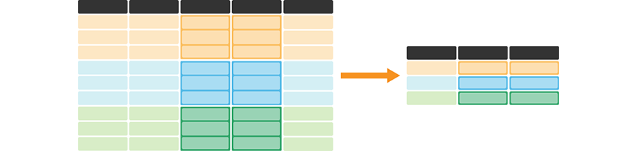
Fig. 3.13 A summary statistic function paired with groupby is useful for calculating that statistic on one or more column(s) for each group. It creates a new data frame with one row for each group and one column for each summary statistic. The darker, top row of each table represents the column headers. The orange, blue, and green colored rows correspond to the rows that belong to each of the three groups being represented in this cartoon example.

The groupby function takes at least one argument—the columns to use in the grouping. Here we use only one column for grouping (region).

region_lang.groupby("region")

<pandas.core.groupby.generic.DataFrameGroupBy object at 0x7f972f0dee10>

Notice that groupby converts a DataFrame object to a DataFrameGroupBy object, which contains information about the groups of the data frame. We can then apply aggregating functions to the DataFrameGroupBy object. Here we first select the most_at_home column, and then summarize the grouped data by their minimum and maximum values using agg.

region_lang.groupby("region")["most_at_home"].agg(["min", "max"])

	min	max
region
Abbotsford - Mission	0	137445
Barrie	0	182390
Belleville	0	97840
Brantford	0	124560
Calgary	0	1065070
...	...	...
Trois-Rivières	0	149835
Vancouver	0	1622735
Victoria	0	331375
Windsor	0	270715
Winnipeg	0	612595

35 rows × 2 columns

The resulting dataframe has region as an index name. This is similar to what happened when we used the pivot function in Section 3.4.2; and just as we did then, you can use reset_index to get back to a regular dataframe with region as a column name.

region_lang.groupby("region")["most_at_home"].agg(["min", "max"]).reset_index()

	region	min	max
0	Abbotsford - Mission	0	137445
1	Barrie	0	182390
2	Belleville	0	97840
3	Brantford	0	124560
4	Calgary	0	1065070
...	...	...	...
30	Trois-Rivières	0	149835
31	Vancouver	0	1622735
32	Victoria	0	331375
33	Windsor	0	270715
34	Winnipeg	0	612595

35 rows × 3 columns

You can also pass multiple column names to groupby. For example, if we wanted to know about how the different categories of languages (Aboriginal, Non-Official & Non-Aboriginal, and Official) are spoken at home in different regions, we would pass a list including region and category to groupby.

region_lang.groupby(["region", "category"])["most_at_home"].agg(["min", "max"]).reset_index()

	region	category	min	max
0	Abbotsford - Mission	Aboriginal languages	0	5
1	Abbotsford - Mission	Non-Official & Non-Aboriginal languages	0	23015
2	Abbotsford - Mission	Official languages	250	137445
3	Barrie	Aboriginal languages	0	0
4	Barrie	Non-Official & Non-Aboriginal languages	0	875
...	...	...	...	...
100	Windsor	Non-Official & Non-Aboriginal languages	0	8235
101	Windsor	Official languages	2695	270715
102	Winnipeg	Aboriginal languages	0	365
103	Winnipeg	Non-Official & Non-Aboriginal languages	0	23565
104	Winnipeg	Official languages	11185	612595

105 rows × 4 columns

You can also ask for grouped summary statistics on the whole data frame.

region_lang.groupby("region").agg(["min", "max"]).reset_index()

	region	category		language		mother_tongue		most_at_home		most_at_work		lang_known
		min	max	min	max	min	max	min	max	min	max	min	max
0	Abbotsford - Mission	Aboriginal languages	Official languages	Aboriginal languages, n.o.s.	Yoruba	0	122100	0	137445	0	93495	0	167835
1	Barrie	Aboriginal languages	Official languages	Aboriginal languages, n.o.s.	Yoruba	0	168990	0	182390	0	115125	0	193445
2	Belleville	Aboriginal languages	Official languages	Aboriginal languages, n.o.s.	Yoruba	0	93655	0	97840	0	54150	0	100855
3	Brantford	Aboriginal languages	Official languages	Aboriginal languages, n.o.s.	Yoruba	0	116645	0	124560	0	73910	0	130835
4	Calgary	Aboriginal languages	Official languages	Aboriginal languages, n.o.s.	Yoruba	0	937055	0	1065070	0	844740	0	1343335
...	...	...	...	...	...	...	...	...	...	...	...	...	...
30	Trois-Rivières	Aboriginal languages	Official languages	Aboriginal languages, n.o.s.	Yoruba	0	147805	0	149835	0	78610	0	149805
31	Vancouver	Aboriginal languages	Official languages	Aboriginal languages, n.o.s.	Yoruba	0	1316635	0	1622735	0	1330555	0	2289515
32	Victoria	Aboriginal languages	Official languages	Aboriginal languages, n.o.s.	Yoruba	0	302690	0	331375	0	211705	0	354470
33	Windsor	Aboriginal languages	Official languages	Aboriginal languages, n.o.s.	Yoruba	0	235990	0	270715	0	166220	0	318540
34	Winnipeg	Aboriginal languages	Official languages	Aboriginal languages, n.o.s.	Yoruba	0	530570	0	612595	0	437460	0	749285

35 rows × 13 columns

If you want to ask for only some columns, for example the columns between "most_at_home" and "lang_known", you might think about first applying groupby and then ["most_at_home":"lang_known"]; but groupby returns a DataFrameGroupBy object, which does not work with ranges inside []. The other option is to do things the other way around: first use ["most_at_home":"lang_known"], then use groupby. This can work, but you have to be careful! For example, in our case, we get an error.

region_lang["most_at_home":"lang_known"].groupby("region").max()

KeyError: "region"

This is because when we use [] we selected only the columns between "most_at_home" and "lang_known", which doesn’t include "region"! Instead, we need to use groupby first and then call [] with a list of column names that includes region; this approach always works.

region_lang.groupby("region")[["most_at_home", "most_at_work", "lang_known"]].max().reset_index()

	region	most_at_home	most_at_work	lang_known
0	Abbotsford - Mission	137445	93495	167835
1	Barrie	182390	115125	193445
2	Belleville	97840	54150	100855
3	Brantford	124560	73910	130835
4	Calgary	1065070	844740	1343335
...	...	...	...	...
30	Trois-Rivières	149835	78610	149805
31	Vancouver	1622735	1330555	2289515
32	Victoria	331375	211705	354470
33	Windsor	270715	166220	318540
34	Winnipeg	612595	437460	749285

35 rows × 4 columns

To see how many observations there are in each group, we can use value_counts.

region_lang.value_counts("region")

region
Abbotsford - Mission                214
St. Catharines - Niagara            214
Québec                              214
Regina                              214
Saguenay                            214
                                   ... 
Kitchener - Cambridge - Waterloo    214
Lethbridge                          214
London                              214
Moncton                             214
Winnipeg                            214
Name: count, Length: 35, dtype: int64

Which takes the normalize parameter to show the output as proportion instead of a count.

region_lang.value_counts("region", normalize=True)

region
Abbotsford - Mission                0.028571
St. Catharines - Niagara            0.028571
Québec                              0.028571
Regina                              0.028571
Saguenay                            0.028571
                                      ...   
Kitchener - Cambridge - Waterloo    0.028571
Lethbridge                          0.028571
London                              0.028571
Moncton                             0.028571
Winnipeg                            0.028571
Name: proportion, Length: 35, dtype: float64

3.10. Apply functions across multiple columns

Computing summary statistics is not the only situation in which we need to apply a function across columns in a data frame. There are two other common wrangling tasks that require the application of a function across columns. The first is when we want to apply a transformation, such as a conversion of measurement units, to multiple columns. We illustrate such a data transformation in Fig. 3.14; note that it does not change the shape of the data frame.

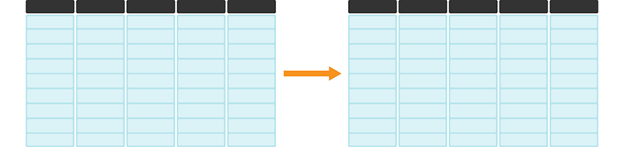
Fig. 3.14 A transformation applied across many columns. The darker, top row of each table represents the column headers.

For example, imagine that we wanted to convert all the numeric columns in the region_lang data frame from int64 type to int32 type using the .astype function. When we revisit the region_lang data frame, we can see that this would be the columns from mother_tongue to lang_known.

region_lang

	region	category	language	mother_tongue	most_at_home	most_at_work	lang_known
0	St. John's	Aboriginal languages	Aboriginal languages, n.o.s.	5	0	0	0
1	Halifax	Aboriginal languages	Aboriginal languages, n.o.s.	5	0	0	0
2	Moncton	Aboriginal languages	Aboriginal languages, n.o.s.	0	0	0	0
3	Saint John	Aboriginal languages	Aboriginal languages, n.o.s.	0	0	0	0
4	Saguenay	Aboriginal languages	Aboriginal languages, n.o.s.	5	5	0	0
...	...	...	...	...	...	...	...
7485	Ottawa - Gatineau	Non-Official & Non-Aboriginal languages	Yoruba	265	65	10	910
7486	Kelowna	Non-Official & Non-Aboriginal languages	Yoruba	5	0	0	0
7487	Abbotsford - Mission	Non-Official & Non-Aboriginal languages	Yoruba	20	0	0	50
7488	Vancouver	Non-Official & Non-Aboriginal languages	Yoruba	190	40	0	505
7489	Victoria	Non-Official & Non-Aboriginal languages	Yoruba	20	0	0	90

7490 rows × 7 columns

We can simply call the .astype function to apply it across the desired range of columns.

region_lang_nums = region_lang.loc[:, "mother_tongue":"lang_known"].astype("int32")
region_lang_nums.info()

<class 'pandas.core.frame.DataFrame'>
RangeIndex: 7490 entries, 0 to 7489
Data columns (total 4 columns):
 #   Column         Non-Null Count  Dtype
---  ------         --------------  -----
 0   mother_tongue  7490 non-null   int32
 1   most_at_home   7490 non-null   int32
 2   most_at_work   7490 non-null   int32
 3   lang_known     7490 non-null   int32
dtypes: int32(4)
memory usage: 117.2 KB

You can now see that the columns from mother_tongue to lang_known are type int32, and that we have obtained a data frame with the same number of columns and rows as the input data frame.

The second situation occurs when you want to apply a function across columns within each individual row, i.e., row-wise. This operation, illustrated in Fig. 3.15, will produce a single column whose entries summarize each row in the original data frame; this new column can be added back into the original data.

Fig. 3.15 A function applied row-wise across a data frame, producing a new column. The darker, top row of each table represents the column headers.

For example, suppose we want to know the maximum value between mother_tongue, and lang_known for each language and region in the region_lang_nums data set. In other words, we want to apply the max function row-wise. In order to tell max that we want to work row-wise (as opposed to acting on each column individually, which is the default behavior), we just specify the argument axis=1.

region_lang_nums.max(axis=1)

0         5
1         5
2         0
3         0
4         5
       ... 
7485    910
7486      5
7487     50
7488    505
7489     90
Length: 7490, dtype: int32

We see that we obtain a series containing the maximum value between mother_tongue, most_at_home, most_at_work and lang_known for each row in the data frame. It is often the case that we want to include a column result from a row-wise operation as a new column in the data frame, so that we can make plots or continue our analysis. To make this happen, we will use column assignment or the assign function to create a new column. This is discussed in the next section.

Note

While pandas provides many methods (like max, astype, etc.) that can be applied to a data frame, sometimes you may want to apply your own function to multiple columns in a data frame. In this case you can use the more general apply method.

3.11. Modifying and adding columns

When we compute summary statistics or apply functions, a new data frame or series is created. But what if we want to append that information to an existing data frame? For example, say we wanted to compute the maximum value in each row of the region_lang_nums data frame, and to append that as an additional column of the region_lang data frame. In this case, we have two options: we can either create a new column within the region_lang data frame itself, or create an entirely new data frame with the assign method. The first option we have seen already in earlier chapters, and is the more commonly used pattern in practice:

region_lang["maximum"] = region_lang_nums.max(axis=1)
region_lang

	region	category	language	mother_tongue	most_at_home	most_at_work	lang_known	maximum
0	St. John's	Aboriginal languages	Aboriginal languages, n.o.s.	5	0	0	0	5
1	Halifax	Aboriginal languages	Aboriginal languages, n.o.s.	5	0	0	0	5
2	Moncton	Aboriginal languages	Aboriginal languages, n.o.s.	0	0	0	0	0
3	Saint John	Aboriginal languages	Aboriginal languages, n.o.s.	0	0	0	0	0
4	Saguenay	Aboriginal languages	Aboriginal languages, n.o.s.	5	5	0	0	5
...	...	...	...	...	...	...	...	...
7485	Ottawa - Gatineau	Non-Official & Non-Aboriginal languages	Yoruba	265	65	10	910	910
7486	Kelowna	Non-Official & Non-Aboriginal languages	Yoruba	5	0	0	0	5
7487	Abbotsford - Mission	Non-Official & Non-Aboriginal languages	Yoruba	20	0	0	50	50
7488	Vancouver	Non-Official & Non-Aboriginal languages	Yoruba	190	40	0	505	505
7489	Victoria	Non-Official & Non-Aboriginal languages	Yoruba	20	0	0	90	90

7490 rows × 8 columns

You can see above that the region_lang data frame now has an additional column named maximum. The maximum column contains the maximum value between mother_tongue, most_at_home, most_at_work and lang_known for each language and region, just as we specified!

To instead create an entirely new data frame, we can use the assign method and specify one argument for each column we want to create. In this case we want to create one new column named maximum, so the argument to assign begins with maximum= . Then after the =, we specify what the contents of that new column should be. In this case we use max just as we did previously to give us the maximum values. Remember to specify axis=1 in the max method so that we compute the row-wise maximum value.

region_lang.assign(
  maximum=region_lang_nums.max(axis=1)
)

	region	category	language	mother_tongue	most_at_home	most_at_work	lang_known	maximum
0	St. John's	Aboriginal languages	Aboriginal languages, n.o.s.	5	0	0	0	5
1	Halifax	Aboriginal languages	Aboriginal languages, n.o.s.	5	0	0	0	5
2	Moncton	Aboriginal languages	Aboriginal languages, n.o.s.	0	0	0	0	0
3	Saint John	Aboriginal languages	Aboriginal languages, n.o.s.	0	0	0	0	0
4	Saguenay	Aboriginal languages	Aboriginal languages, n.o.s.	5	5	0	0	5
...	...	...	...	...	...	...	...	...
7485	Ottawa - Gatineau	Non-Official & Non-Aboriginal languages	Yoruba	265	65	10	910	910
7486	Kelowna	Non-Official & Non-Aboriginal languages	Yoruba	5	0	0	0	5
7487	Abbotsford - Mission	Non-Official & Non-Aboriginal languages	Yoruba	20	0	0	50	50
7488	Vancouver	Non-Official & Non-Aboriginal languages	Yoruba	190	40	0	505	505
7489	Victoria	Non-Official & Non-Aboriginal languages	Yoruba	20	0	0	90	90

7490 rows × 8 columns

This data frame looks just like the previous one, except that it is a copy of region_lang, not region_lang itself; making further changes to this data frame will not impact the original region_lang data frame.

As another example, we might ask the question: “What proportion of the population reported English as their primary language at home in the 2016 census?” For example, in Toronto, 3,836,770 people reported speaking English as their primary language at home, and the population of Toronto was reported to be 5,928,040 people. So the proportion of people reporting English as their primary language in Toronto in the 2016 census was 0.65. How could we figure this out starting from the region_lang data frame?

First, we need to filter the region_lang data frame so that we only keep the rows where the language is English. We will also restrict our attention to the five major cities in the five_cities data frame: Toronto, Montréal, Vancouver, Calgary, and Edmonton. We will filter to keep only those rows pertaining to the English language and pertaining to the five aforementioned cities. To combine these two logical statements we will use the & symbol. and with the [] operation, "English" as the language and filter the rows, and name the new data frame english_langs.

english_lang = region_lang[
    (region_lang["language"] == "English") &
    (region_lang["region"].isin(five_cities["region"]))
]
english_lang

	region	category	language	mother_tongue	most_at_home	most_at_work	lang_known
1898	Montréal	Official languages	English	444955	620510	412120	2500590
1903	Toronto	Official languages	English	3061820	3836770	3218725	5600480
1918	Calgary	Official languages	English	937055	1065070	844740	1343335
1919	Edmonton	Official languages	English	930405	1050410	792700	1275265
1923	Vancouver	Official languages	English	1316635	1622735	1330555	2289515

Okay, now we have a data frame that pertains only to the English language and the five cities mentioned earlier. In order to compute the proportion of the population speaking English in each of these cities, we need to add the population data from the five_cities data frame.

five_cities

	region	households	area	population	dwellings
29	Edmonton	502143	9857.77908	1321426	537634
31	Calgary	519693	5241.70103	1392609	544870
32	Vancouver	960894	3040.41532	2463431	1027613
33	Montréal	1727310	4638.24059	4098927	1823281
34	Toronto	2135909	6269.93132	5928040	2235145

The data frame above shows that the populations of the five cities in 2016 were 5928040 (Toronto), 4098927 (Montréal), 2463431 (Vancouver), 1392609 (Calgary), and 1321426 (Edmonton). Next, we will add this information to a new data frame column called city_pops. Once again, we will illustrate how to do this using both the assign method and regular column assignment. We specify the new column name (city_pops) as the argument, followed by the equals symbol =, and finally the data in the column. Note that the order of the rows in the english_lang data frame is Montréal, Toronto, Calgary, Edmonton, Vancouver. So we will create a column called city_pops where we list the populations of those cities in that order, and add it to our data frame. And remember that by default, like other pandas functions, assign does not modify the original data frame directly, so the english_lang data frame is unchanged!

english_lang.assign(
  city_pops=[4098927, 5928040, 1392609, 1321426, 2463431]
)

	region	category	language	mother_tongue	most_at_home	most_at_work	lang_known	city_pops
1898	Montréal	Official languages	English	444955	620510	412120	2500590	4098927
1903	Toronto	Official languages	English	3061820	3836770	3218725	5600480	5928040
1918	Calgary	Official languages	English	937055	1065070	844740	1343335	1392609
1919	Edmonton	Official languages	English	930405	1050410	792700	1275265	1321426
1923	Vancouver	Official languages	English	1316635	1622735	1330555	2289515	2463431

Instead of using the assign method we can directly modify the english_lang data frame using regular column assignment. This would be a more natural choice in this particular case, since the syntax is more convenient for simple column modifications and additions.

english_lang["city_pops"] = [4098927, 5928040, 1392609, 1321426, 2463431]
english_lang

/tmp/ipykernel_12/2654974267.py:1: SettingWithCopyWarning:
A value is trying to be set on a copy of a slice from a DataFrame.
Try using .loc[row_indexer,col_indexer] = value instead

See the caveats in the documentation: https://pandas.pydata.org/pandas-docs/stable/user_guide/indexing.html#returning-a-view-versus-a-copy
  english_lang["city_pops"] = [4098927, 5928040, 1392609, 1321426, 2463431]

	region	category	language	mother_tongue	most_at_home	most_at_work	lang_known	city_pops
1898	Montréal	Official languages	English	444955	620510	412120	2500590	4098927
1903	Toronto	Official languages	English	3061820	3836770	3218725	5600480	5928040
1918	Calgary	Official languages	English	937055	1065070	844740	1343335	1392609
1919	Edmonton	Official languages	English	930405	1050410	792700	1275265	1321426
1923	Vancouver	Official languages	English	1316635	1622735	1330555	2289515	2463431

Wait a moment…what is that warning message? It seems to suggest that something went wrong, but if we inspect the english_lang data frame above, it looks like the city populations were added just fine! As it turns out, this is caused by the earlier filtering we did from region_lang to produce the original english_lang. The details are a little bit technical, but pandas sometimes does not like it when you subset a data frame using [] or loc[] followed by column assignment. For the purposes of your own data analysis, if you ever see a SettingWithCopyWarning, just make sure to double check that the result of your column assignment looks the way you expect it to before proceeding. For the rest of the book, we will silence that warning to help with readability.

Note

Inserting the data column [4098927, 5928040, ...] manually as we did above is generally very error-prone and is not recommended. We do it here to demonstrate another usage of assign and regular column assignment. But in more advanced data wrangling, one would solve this problem in a less error-prone way using the merge function, which lets you combine two data frames. We will show you an example using merge at the end of the chapter!

Now we have a new column with the population for each city. Finally, we can convert all the numerical columns to proportions of people who speak English by taking the ratio of all the numerical columns with city_pops. Let’s modify the english_lang column directly; in this case we can just assign directly to the data frame. This is similar to what we did in Section 3.4.3, when we first read in the "region_lang_top5_cities_messy.csv" data and we needed to convert a few of the variables to numeric types. Here we assign to a range of columns simultaneously using loc[]. Note that it is again possible to instead use the assign function to produce a new data frame when modifying existing columns, although this is not commonly done. Note also that we use the div method with the argument axis=0 to divide a range of columns in a data frame by the values in a single column—the basic division symbol / won’t work in this case.

english_lang.loc[:, "mother_tongue":"lang_known"] = english_lang.loc[
    :,
    "mother_tongue":"lang_known"
    ].div(english_lang["city_pops"], axis=0)
english_lang

	region	category	language	mother_tongue	most_at_home	most_at_work	lang_known	city_pops
1898	Montréal	Official languages	English	0.108554	0.151384	0.100543	0.610060	4098927
1903	Toronto	Official languages	English	0.516498	0.647224	0.542966	0.944744	5928040
1918	Calgary	Official languages	English	0.672877	0.764802	0.606588	0.964617	1392609
1919	Edmonton	Official languages	English	0.704092	0.794906	0.599882	0.965067	1321426
1923	Vancouver	Official languages	English	0.534472	0.658730	0.540123	0.929401	2463431

3.12. Using merge to combine data frames

Let’s return to the situation right before we added the city populations of Toronto, Montréal, Vancouver, Calgary, and Edmonton to the english_lang data frame. Before adding the new column, we had filtered region_lang to create the english_lang data frame containing only English speakers in the five cities of interest.

english_lang

	region	category	language	mother_tongue	most_at_home	most_at_work	lang_known
1898	Montréal	Official languages	English	444955	620510	412120	2500590
1903	Toronto	Official languages	English	3061820	3836770	3218725	5600480
1918	Calgary	Official languages	English	937055	1065070	844740	1343335
1919	Edmonton	Official languages	English	930405	1050410	792700	1275265
1923	Vancouver	Official languages	English	1316635	1622735	1330555	2289515

We then added the populations of these cities as a column (Toronto: 5928040, Montréal: 4098927, Vancouver: 2463431, Calgary: 1392609, and Edmonton: 1321426). We had to be careful to add those populations in the right order; this is an error-prone process. An alternative approach, that we demonstrate here is to (1) create a new data frame with the city names and populations, and (2) use merge to combine the two data frames, recognizing that the “regions” are the same.

We create a new data frame by calling pd.DataFrame with a dictionary as its argument. The dictionary associates each column name in the data frame to be created with a list of entries. Here we list city names in a column called "region" and their populations in a column called "population".

city_populations = pd.DataFrame({
  "region" : ["Toronto", "Montréal", "Vancouver", "Calgary", "Edmonton"],
  "population" : [5928040, 4098927, 2463431, 1392609, 1321426]
})
city_populations

	region	population
0	Toronto	5928040
1	Montréal	4098927
2	Vancouver	2463431
3	Calgary	1392609
4	Edmonton	1321426

This new data frame has the same region column as the english_lang data frame. The order of the cities is different, but that is okay! We can use the merge function in pandas to say we would like to combine the two data frames by matching the region between them. The argument on="region" tells pandas we would like to use the region column to match up the entries.

english_lang = english_lang.merge(city_populations, on="region")
english_lang

	region	category	language	mother_tongue	most_at_home	most_at_work	lang_known	population
0	Montréal	Official languages	English	444955	620510	412120	2500590	4098927
1	Toronto	Official languages	English	3061820	3836770	3218725	5600480	5928040
2	Calgary	Official languages	English	937055	1065070	844740	1343335	1392609
3	Edmonton	Official languages	English	930405	1050410	792700	1275265	1321426
4	Vancouver	Official languages	English	1316635	1622735	1330555	2289515	2463431

You can see that the populations for each city are correct (e.g. Montréal: 4098927, Toronto: 5928040), and we can proceed to with our analysis from here.

3.13. Summary

Cleaning and wrangling data can be a very time-consuming process. However, it is a critical step in any data analysis. We have explored many different functions for cleaning and wrangling data into a tidy format. Table 3.4 summarizes some of the key wrangling functions we learned in this chapter. In the following chapters, you will learn how you can take this tidy data and do so much more with it to answer your burning data science questions!

Table 3.4 Summary of wrangling functions

Function	Description
agg	calculates aggregated summaries of inputs
assign	adds or modifies columns in a data frame
groupby	allows you to apply function(s) to groups of rows
iloc	subsets columns/rows of a data frame using integer indices
loc	subsets columns/rows of a data frame using labels
melt	generally makes the data frame longer and narrower
merge	combine two data frames
pivot	generally makes a data frame wider and decreases the number of rows
str.split	splits up a string column into multiple columns

3.14. Exercises

Practice exercises for the material covered in this chapter can be found in the accompanying worksheets repository in the “Cleaning and wrangling data” row. You can launch an interactive version of the worksheet in your browser by clicking the “launch binder” button. You can also preview a non-interactive version of the worksheet by clicking “view worksheet.” If you instead decide to download the worksheet and run it on your own machine, make sure to follow the instructions for computer setup found in Chapter 13. This will ensure that the automated feedback and guidance that the worksheets provide will function as intended.

3.15. Additional resources

• The pandas package documentation is another resource to learn more about the functions in this chapter, the full set of arguments you can use, and other related functions.

• Python for Data Analysis [McKinney, 2012] has a few chapters related to data wrangling that go into more depth than this book. For example, the data wrangling chapter covers tidy data, melt and pivot, but also covers missing values and additional wrangling functions (like stack). The data aggregation chapter covers groupby, aggregating functions, apply, etc.

• You will occasionally encounter a case where you need to iterate over items in a data frame, but none of the above functions are flexible enough to do what you want. In that case, you may consider using a for loop [McKinney, 2012].

3.16. References

McK12(1,2)

Wes McKinney. Python for data analysis: Data wrangling with Pandas, NumPy, and IPython. " O'Reilly Media, Inc.", 2012.

Wic14

Hadley Wickham. Tidy data. Journal of Statistical Software, 59(10):1–23, 2014.